Sidebar
<latex>{\fontsize{16pt}\selectfont \textbf{Nonlinear MPC for Robotic Arms}} </latex>
<latex>{\fontsize{12pt}\selectfont \textbf{Brahayam Pontón}} </latex>
<latex>{\fontsize{10pt}\selectfont \textit{Semester Project RSC}} </latex>
<latex> {\fontsize{12pt}\selectfont \textbf{Abstract} </latex>
Differential Dynamic Programming, known as DDP, is a trajectory optimization algorithm used for determining optimal control policies for a nonlinear system. It is based on applying the Principle of Optimality around nominal trajectories, and iteratively computing improved trajectories.
The aim of this semester project is to use this technique to control a planar robotic arm of n-links and evaluate its performance, scalability of the algorithm for high number of degrees of freedom and real time constraints, and analyze suitability for the use on real robots where no perfect model of the robot and environment is available.
<latex> {\fontsize{12pt}\selectfont \textbf{How does DDP work?} </latex>
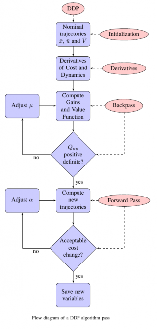
Differential Dynamic Programming is a numerical technique which does not look for a global optimal control policy, but instead, it is based on a second order approximation of the value function for determining optimal control policies for the current state. It has 3 basic steps:
- Calculation of Derivatives: The first and second derivatives of the dynamics of the system we want to control, and of a cost function, we wish to minimize, along a nominal state and control trajectories are needed.
- Backward Pass: In this step, the pre-computed derivatives are used to approximate the value function and to compute an affine approximation of the locally optimal control law, given by an open and a closed loop gains.
- Forward Pass: In this step, the computed gains are applied to the system taking as reference the nominal trajectories. If there has been an improvement in the performance index of the optimal control problem, the new trajectories are accepted and improved iteratively until some tolerance parameter.
<latex> {\fontsize{12pt}\selectfont \textbf{Some Improvements to DDP} </latex>
The improvements to be presented, were proposed in 1):
- Regularization: DDP is based on a second order Taylor approximation of the real value function. In order to keep this approximation valid, the variations of the considered parameters around the nominal values should be kept small. This improvement consists in keeping the variations in the state close to the current nominal values by applying a quadratic cost to the nominal state trajectory. This improves the robustness of the algorithm.
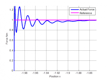
- Line Search: This improvement makes the algorithm faster, because it helps to find a feasible control solution, taking into account the new states during the integration process in the forward pass. It speeds up the process of getting a solution, because we have the opportunity of finding a feasible control sequence without having to re-compute the derivatives in a new iteration.
| <latex> {\fontsize{12pt}\selectfont \textbf{Plant to be controlled} </latex> | <latex> {\fontsize{12pt}\selectfont \textbf{Cost Function} </latex> |
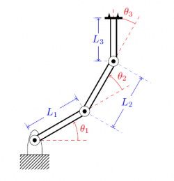
| This algorithm is model-based, therefore, we need to explicitly formulate a description of the dynamics of the system, we are aiming to control. In this project, we used a planar robotic arm of n-links. | The cost function must contain the objectives that we are willing to achieve. The function used for evaluating the cost is given by: |
M(q) \ddot q + V(q,\dot q) + G(q) = \Gamma \end{equation*} where $q$ are the Generalized Joint Coordinates, $M(q)$ is the Mass matrix, $V(q,\dot q)$ is the Coriolis and Centrifugal forces matrix, $G(q)$ is the Gravity matrix and $\Gamma$ is the vector of Generalized forces. |\begin{equation*} \begin{split} \label{eq_cst_4} \ell (\textbf{x}, \textbf{u}, i) &= cost_X[x_i - x_t]^2 + cost_U[u_i]^2 \\* &+ cost_O \sum\limits_{j=1}^{obs} \mathcal{N} (x_i; x_j,\Sigma) \\* &+ cost_S \mathcal{N} (svx_i; 0,\sigma^2) \\* \end{split} \end{equation*} |
<latex> {\fontsize{12pt}\selectfont \textbf{Some Results} </latex>
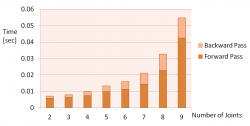
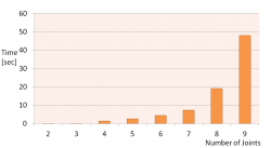
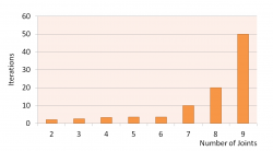
The computational complexity for the derivatives is $\sim \BigO {N n^5}$, for the backward and forward passes $\sim \BigO {N n^3}$; where $N$ represents the number of timesteps used in the receding time horizon given by $N = Simulation Time / dt$. The other variable is $n$ which represents the dimension of the state vector of the dynamics. This shows that the biggest effort is in the compulation of the derivatives, as can be seen in the following figures.
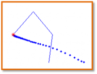
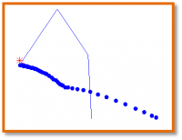
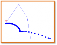
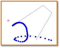
It was also explored that DDP can easily handle model error regarding the mass and inertia properties. DDP is not sensitive to modelling errors in the mass and inertia properties of the several links. However, it is not able to handle appropriately errors in the length of the links. This means that the kinematic model should be accurate. The following Figures show the results for Go-to-Goal motion for the indicated errors in length. Numerical results can be found in the report.
| 1% model error in length | 10% model error in length | 20% model error in length | 50% model error in length |
|---|---|---|---|
 |  |  |  |
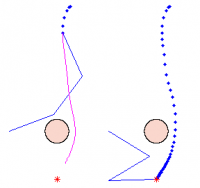 | A remarkable result of DDP is that it can easily incorporate the description of obstacles in the cost function and in this way, it can plan in environments with static and dynamic obstacles. |
<latex> {\fontsize{12pt}\selectfont \textbf{Conclusions} </latex>
- Differential Dynamic Programming is a robust and reliable method, that can manage a large class of nonlinear problems, but it is relatively complex to implement and computationally demanding.
- DDP overcomes, to a large extent, the curse of dimensionality, by looking not for global optimal solutions, but for solutions that satisfy Bellman`s equation from an admissible control set.
- This method could be easily extended to incorporate control constraints and state constraints.
<latex> {\fontsize{12pt}\selectfont \textbf{Further Work} </latex>
- An study of force control with DDP by solving the Stochastic Complementarity Problem as suggested in 2) and a comparison between this approach and a hybrid-automaton based approach would be of interest for further work.
- It is also important to write an efficient implementation for the computation of the derivatives and test if it would be really possible to use DDP for real-time applications.
- The concept of gap metric used in nonlinear control could be applied to this problem, in order to compare the linearized model to the full nonlinear model; with the objective of getting an idea of how good or bad the linearization around an operating point represents the model in the neighborhood of the nominal operating point. This would be useful to determine if the criterion used for the selection of the applied control gains to the system is correct or could be improved.
- It could also be of interest to test the performance of DDP in whole body obstacle avoidance problem and compare with an iterative learning method for control.

