LAB

<latex>{\fontsize{16pt}\selectfont \textbf{Partial Differential Flatness in HyQ}} </latex>

<latex>{\fontsize{12pt}\selectfont \textbf{Carmelo Sferrazza}} </latex>
<latex>{\fontsize{10pt}\selectfont \textit{Semester Project, RSC}} </latex>

<latex> {\fontsize{12pt}\selectfont \textbf{Abstract} </latex>

One of the challenges that robotics has been facing in the last years is the generation of dynamically feasible trajectories for any general underactuated robotic system. This generation process involves a constrained nonlinear optimization problem and it requires numerical integration to choose a feedforward input in order to obtain the desired trajectories for the system states¹⁾, and for high-dimensional systems this problem can be very time-consuming.
Nevertheless, for a small class of systems, called differentially flat, the trajectory generation process can be simplified: in some cases, as it will be shown in the following, the problem reduces to solving a linear system of equations.
However, most underactuated systems are not differentially flat, so a broader class of systems have been proposed and called partially differentially flat²⁾.

<latex> {\fontsize{12pt}\selectfont \textbf{Background} </latex>

A system $\dot{x}(t) = f(x(t),u(t))$, $x \in \mathbb R^n$, $u \in \mathbb R^m$, is partially differentially flat ³⁾ if there exists a partition of the states, $ x = \begin{bmatrix} x^r
x^{ur} \end{bmatrix} $, $x^r \in \mathbb R^k$, $x^{ur} \in \mathbb R^{n-k}$, $k \leq n$ (called retrievable states and unretrievable states), and there exist “flat” outputs $y\in \mathbb R^m$, function of the retrievable states, the inputs and the derivatives of the latters, such that the retrievable states and all the inputs can be expressed as a function of the flat outputs and a finite number of their derivatives, and the unretrievable states dynamics are those of one or more chains of integrators. Moreover, the derivative of the last elements of each of these chains can also be expressed as a function of the flat outputs and their derivatives.
In mathematical notation, there exist functions $F, G, H$, finite integers $p,q,l$, matrices $A_i$ and $b_i$ for $i = 1,\cdots,l$, such that:

$y = F(s,u,\dot{u},\cdots,u^{(p)}) $
$x^r = G(y, \dot{y},\cdots,y^{(q)})$
$u = H(y, \dot{y},\cdots,y^{(q)})$

$\dot{x}^{ur} = \begin{bmatrix} A_1 & \textbf{0} & \cdots & \textbf{0}
\textbf{0} & A_2 & \cdots & \textbf{0}
\vdots & \vdots & \ddots & \vdots
\textbf{0} & \textbf{0} & \cdots & A_l \end{bmatrix} x^{ur} + \begin{bmatrix} b_1
b_2
\vdots
b_l \end{bmatrix}$

where $l$ is the number of chains of integrators, and $A_i$ and $b_i$ are given as:
$A_i = \begin{bmatrix} \textbf{0} & \textbf{I}
0 & \textbf{0} \end{bmatrix}\;, \quad b_i = \begin{bmatrix} \textbf{0}
h_i(y,\dot{y},\cdots,y^{(q)}) \end{bmatrix}$
where $h_i$ is a smooth scalar function. $\textbf{0}$ represents zero vectors/matrices of appropriate dimensions, and $\textbf{I}$ is the identity matrix, also of appropriate dimensions.

<latex> {\fontsize{12pt}\selectfont \textbf{Partial Differential Flatness on the Planar Ballbot} </latex>

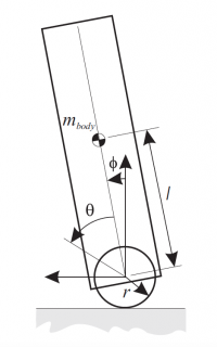
The following equations of motion represent the model above:

$M(q)\ddot{q} + H(q,\dot{q}) = \begin{bmatrix} 0
\tau \end{bmatrix}$

$q = \begin{bmatrix} \phi
\theta \end{bmatrix}\;, \quad M(q) = \begin{bmatrix} \alpha + \gamma + 2\beta cos(\phi) & \alpha + \beta cos(\phi)
\alpha + \beta cos(\phi) & \alpha \end{bmatrix}$

$H(q,\dot{q}) = \begin{bmatrix} -\beta sin(\phi) \dot{\phi}^2 - \frac{\beta g }{r} sin(\phi)
-\beta sin(\phi) \dot{\phi}^2 \end{bmatrix}$

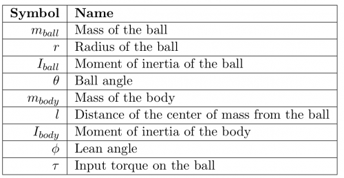
with: $\alpha = I_{ball} + (m_{ball}+m_{body})r^2$, $\beta = m_{body}rl$, $\gamma = I_{body}+m_{body}l^2$.

Defining the flat output as $y = \phi$, and the states as $x = \begin{bmatrix}x^{ur}
x^r\end{bmatrix}$, with $x^{ur} = \begin{bmatrix}\theta
\dot{\theta}\end{bmatrix}$ and $x^r = \begin{bmatrix}\phi
\dot{\phi}\end{bmatrix}$, the following relations can be derived:

$\phi = y \;, \quad \dot{\phi} = \dot{y}$

$\ddot{\theta} = h(y,\dot{y},\ddot{y})= \dfrac{\beta sin(y) \dot{y}^2 + \frac{\beta g sin(y)}{r} - [\alpha + \gamma + 2\beta cos(y)]\ddot{y}}{\alpha + \beta cos(y)}$

$\tau = \alpha h(y,\dot{y},\ddot{y}) + [\alpha + \beta cos(y)]\ddot{y} - \beta sin(y) \dot{y}^2 = g(y,\dot{y},\ddot{y})$

Therefore, the retrievable states, the input and $\ddot{\theta}$ can be retrieved from the flat output and its derivatives. Moreover, the dynamics of the unretrievable states is the one of a chain of integrators:
$\dot{x^{ur}} = \begin{bmatrix} \dot{\theta}
\ddot{\theta} \end{bmatrix} = A\begin{bmatrix} \theta
\dot{\theta} \end{bmatrix} + b$

$A = \begin{bmatrix} 0 & 1
0 & 0 \end{bmatrix} \;, \quad b = \begin{bmatrix} 0
h(y,\dot{y}, \ddot{y}) \end{bmatrix}$

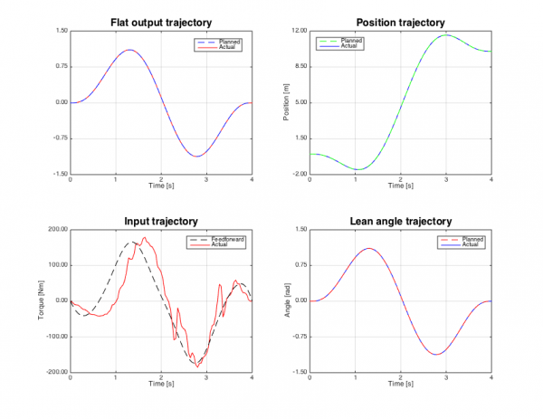
After solving an optimization problem, a simulation of the system (no constraints on states and input) has been performed using a Time-Varying LQR, with the goal to go from 0 to 10m in 4s. The results are shown in the tracking plots and in the video below. We have shown that this approach is faster than standard nonlinear optimization techniques.

<latex> {\fontsize{12pt}\selectfont \textbf{Numerical search} </latex>

Finding the flat outputs is not always as simple as in the ballbot example. Moreover, the functions connecting these flat outputs with the states and the inputs are often hard to derive. Therefore, proving partial differential flatness on high-dimensional systems, or on systems of which only a numerical model is available (i.e. derived from algorithms), can be very difficult.
In the following, a numerical procedure is shown in order to prove partial differential flatness on a system, approximately finding the flat outputs and the desired functions.
The main assumption is that a collection of trajectories is available for the analyzed system. Therefore, partial differential flatness is proved around these trajectories.

We have proposed this numerical search for both Differential Flatness (D.F.) and Partial Differential Flatness (P.D.F.). \\Regarding P.D.F., using the notation of the definition, the following assumptions have been made:
- The states are a set of $\frac{n}{2}$ chains of integrators of length 2 (i.e. $x = [q \hspace{1mm} \dot{q}]^T$), therefore we want to satisfy $\ddot{q}_{ur} = \begin{bmatrix} h_1(y,\dot{y},\cdots,y^{(\mu)})
\vdots \\h_{\frac{n_{ur}}{2}}(y,\dot{y},\cdots,y^{(\mu)})\end{bmatrix}$, where $q_{ur}$ groups the first elements of each chain of integrators related to the unretrievable states.
- $F$ is a linear combination of some basis functions of the retrievable states.
- $G$, $H$ and $h_i$ are linear combinations of some basis functions of $y$ and a defined finite number $\mu$ of its derivatives. Based on these, the following nonlinear problem has to be solved: \begin{equation*} \begin{aligned} & \underset{}{\text{find}} & & P, Q, K, J
& \text{subject to} & & y(t) = P\mathcal{X}^{r*}(t)
& & & u^*(t) = Q\mathcal{Y}(t)
& & & s^*(t) = K\mathcal{Y}(t)
& & & \ddot{q}_{ur}^*(t) = J\mathcal{Y}(t)
\end{aligned} \end{equation*}
where $x = \begin{bmatrix} x^{ur}
x^r \end{bmatrix}$, $x^{ur} \in \mathbb R^{n_{ur}}$, $x^r \in \mathbb R^{n_r}$, $\mathcal{X}^r$ is a vector of dimension $\eta$ containing basis functions of $x^r$ and $\mathcal{Y}$ is a vector of dimension $\nu$ containing basis functions of $y$ and its first $\mu$ derivatives (i.e. $\mathcal{Y} = [y\hspace{1mm} \dot{y} \hspace{1mm}\ddot{y}]^T$), $P \in \mathbb R^{m \textrm{x} \eta}$, $Q \in \mathbb R^{m \textrm{x} \nu}$, $K \in \mathbb R^{n_r \textrm{x} \nu}$ and $J \in \mathbb R^{\frac{n_{ur}}{2} \textrm{x} \nu}$. The partition of the states has to be determined solving the program using different combinations of the chains of integrators among the unretrievable states and the retrievable states.
Once appropriate non-zero matrices $P$, $Q$, $K$, $J$ have been found within certain error limits for a collection of trajectories, it is possible to state that the system is partially differentially flat around these trajectories, with flat outputs $y = P\mathcal{X}^r$.

<latex> {\fontsize{12pt}\selectfont \textbf{Partial Differential Flatness on Floating Base Robots} </latex>
Finally, P.D.F. has been proved on a floating base quaduped (e.g. HyQ). To do this, two of the legs have been assumed to stay still around a fixed position.
The idea in the following has been to plan the velocities of the “chosen” joints (the moving joints and the degrees of freedom of the base) as third order hermitian splines with a method inspired by Direct Collocation ⁴⁾. The time range is divided into a finite number of intervals, and the values of the acceleration of the chosen joints at the extrema (called nodes) and at the middle points (called collocation points) of these intervals are the decision variables. Since we are dealing with third order splines, the Simpson's rule has been used for the integration of the accelerations, and subsequently, making an approximation, for the integration of the velocities.

The constraint that two of the legs have to remain still has to be verified in the optimization process only at the nodes (and at the collocation points), assuming that the velocity of such legs is a trapezoidal spline.
The P.D.F. of the system makes it possible to leave the input out of the decision variables.
In the following video, a simulation of the robot (no constraints on the torques and joint velocities) turning of $\frac{\pi}{2}$ around its yaw in 3 seconds is shown.