LAB

<latex>{\fontsize{16pt}\selectfont \textbf{Agile Flight with a Cable-Suspended Load}} </latex>

<latex>{\fontsize{12pt}\selectfont \textbf{Cédric de Crousaz}} </latex>
<latex>{\fontsize{10pt}\selectfont \textit{Semester Project RSC}} </latex>

<latex> {\fontsize{12pt}\selectfont \textbf{Abstract} </latex>

Motion control learning is one of the founding blocks for any robotic system. For simple systems, dynamic programming can be used to find globally optimal control trajectories. However, for highly nonlinear, high dimensional systems, the generation of such trajectories through dynamic programming is no longer feasible, and other, possibly locally optimal methods need to be used.
In this thesis, the iterative LQG (iLQG) algorithm is used to find control trajectories for a quadrotor with a cable-suspended load. This relatively high-dimensional, highly nonlinear system with several degrees of underactuation and even hybrid dynamics solved different tasks using this algorithm. In particular, the quadrotor was required to pass through a small window, too small for the load to remain in a vertical, taut, state. The ultimate goal of this project is to provide good initial trajectories for a learning algorithm such as <latex> PI$^2$-01 </latex>, enable robots to learn and correct their control trajectories and/or system models in an autonomous way.

<latex> {\fontsize{12pt}\selectfont \textbf{iLQG Algorithm} </latex>

The iterative Linear Quadratic Gaussian (iLQG) method presented by Todorov et al¹⁾ returns a locally optimal linear feedback controller for arbitrary nonlinear systems and nonquadratic lowerbounded cost functions. The optimal control is found by minimizing a cost function \begin{equation} J = \E \left[ h( \textbf{x}(t_f)) ) + \textstyle{\sum_{t = 0}^{t_f-1} } l(t,\textbf{x}(t),\textbf{u}(t)) \right] \label{eq:ilqg_cost} \end{equation}

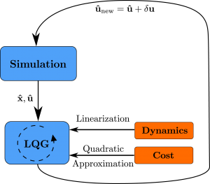
where $h( \textbf{x}(t_f) )$ is the penalty on the state $\textbf{x}$ at the final time $t_f$, and $l(t,\textbf{x},\textbf{u})$ is an immediate penalty in each time step. The main steps of the algorithm are described in the figure on the right. The starting point is an initial nominal trajectory, generated in this case using a stabilizing LQR controller. In each time step, the system is then linearized around this nominal trajectory and a quadratic approximation of the cost is used. Each iteration then yields a new control trajectory, which can then be fed back into the system to obtain a new nominal state trajectory.

<latex> {\fontsize{12pt}\selectfont \textbf{Hybrid Model} </latex>

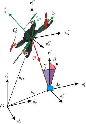
The system shown on the right consists of a quadrotor with mass $m_Q = 0.5\,[kg]$ and moment of inertia $\vI_Q = diag(0.03,0.03, 0.05)\, [kg\,m^2]$, from which a load with mass $m_L = 50\,[g]$ is hung by a massless cable of length $L_c = 1\,[m]$.

As the cable can only handle tensile forces along the direction of the string, this is a hybrid system with two different system dynamics, referred to as modes. In the first mode, the cable is taut and transferring a force between load and quadrotor, while in the second, there is no tension in the cable and the load is in free fall.

A transition between the system modes happens whenever the state trajectory intersects with one of the switching surfaces. The free fall mode is entered when the tension in the cable vanishes, which is represented by the switching surface $$\mathcal{S}_1 &= \{ \textbf{x} \, | \, F_c = m_L \left( \ddot{\textbf{x}}_L + g\, \ve_3 \right) \cdot \textbf{p} \equiv 0 \}$$ where $\textbf{x}_L$ is the position vector of the load, and $\textbf{p}$ is a unit vector point from the center of mass of the quadrotor to the load. As soon as the load moves away from the quadrotor and has reached the distance $r = L_c$ from the center of mass of the quadrotor, represented by $$\mathcal{S}_2 = \{ \textbf{x} \, | \, | r | = L_c, \, \frac{d}{dt}r > 0 \}$$ the tension inside the cable is non-zero again, and the taut mode is entered again.

<latex> {\fontsize{12pt}\selectfont \textbf{Cost Function} </latex>

The cost function in $(1)$ was defined by quadratic penalties on both the deviation of the state from the equilibrium position (for stability) and on the input (for a finite solution). In addition, a term $g(t,\textbf{x},\textbf{u})$ was added to the immediate cost to shape the individual tasks. More precisely, this additional cost term was constructed using sums of waypoint functions of the form $$C(t_p,\textbf{x}_p, \textbf{W}_p,\rho) = \left( \textbf{x} - \textbf{x}_p \right)^\top \textbf{W}_p \left( \textbf{x} - \textbf{x}_p \right)\cdot \sqrt{\frac{\rho}{2 \pi}} exp\left( - \frac{\rho}{2} (t - t_p)^2 \right)$$ putting a quadratic penalty on the deviation from desired states $\textbf{x}_p$ at time $t_p$, spread over time by a Gaussian shaped by the parameter $\rho$.

<latex> {\fontsize{12pt}\selectfont \textbf{Results} </latex>

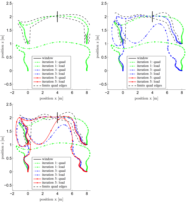
Different tasks were successfully performed using the iLQG algorithm and the cost function structure presented above. For one of these tasks, the quadrotor is told to pass a small window of height $w_h = 0.4 L_c$ and width $w_w = 0.6 L_c$ by letting the load fly through first. This is achieved by penalizing the deviation of the load and quadrotor from the window center at a particular time, at which the string is requested to be in a horizontal position.

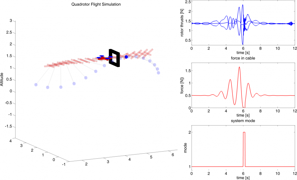
The results after the first, third and fifth iteration starting from the stabilizing LQR trajectory is displayed on the right. In the figure below, a shaded simulation of the result after the fifth iteration is shown. In addition, the three plots on the right show the rotor thrusts, the force in the cable and the system mode. Mode $1$ means the cable is taut, whereas in mode $2$, the load is in free fall. Note that there is a mode switch when the load passes the window, i.e. the force in the cable vanishes at $t = 6\,[s]$, so the load is in free fall and the system transitions into mode $2$. After passing the window, the load is caught again by the quadrotor and tension is once again present in the cable. This shows that, in the tasks at hand, the controller is able to handle mode switches in the trajectory. High quality videos for this and other tasks can be found at High quality videos of tasks

The challenge with this approach is that the iLQG algorithm can diverge, in particular when a highly non-quadratic cost is used or the input saturation bounds are violated heavily. In these cases, the result has to be approached gradually by first using a simpler cost function leading into the right direction, and then using the resulting trajectory to initialize a more complex cost function.

<latex> {\fontsize{12pt}\selectfont \textbf{Conclusion and Future Works} </latex>

The iLQG method was applied to a hybrid system consisting of a quadrotor with suspended load. In the simulations presented, the switching between the modes is handled well by the algorithm, but small stepwise changes of the penalty weights may be necessary to avoid divergence of iLQG. In a next step, the unmodelled dynamics need to be addressed. One possible approach which will be pursued is to apply the iLQG trajectory to a learning algorithm such as <latex> PI$^2$-01 </latex> similarly to ²⁾, adjusting a good initial solution to the model inaccuracies.