Sidebar
<latex>{\fontsize{16pt}\selectfont \textbf{Visual-Inertial State Estimation for Visual Servoing}} </latex>
<latex>{\fontsize{12pt}\selectfont \textbf{Christoph Zumbrunn}} </latex>
<latex>{\fontsize{10pt}\selectfont \textit{Master Project ME}} </latex>
<latex> {\fontsize{12pt}\selectfont \textbf{Abstract} </latex>
 The In-Situ Fabricator (IF) was designed to perform common tasks on a building construction site such as placing bricks or painting walls which requires a high precision. However, the end-effector pose of the robot is not known accurately due to base tilt and joint tolerances.
The goal of this master project is to fuse visual and inertial data in a state estimation algorithm to get an accurate prediction of the end-effector pose in real time. The algorithm was tested using movements of a robotic arm in a sandbox simulation as well as experiments with the VI sensor hardware. The results are compared to data recorded using an indoor GPS solution. IMU and visual data have been fused to estimate a trajectory spanning 0.5 seconds at 50 Hz. Although the algorithm can handle a short loss of visual contact to the target, it diverges quickly from the true pose. The framework was designed to consist of an application-independent layer to solve a general batch estimation problem (which can be used for other projects as well) and an application-specific ROS node for the given task.
<latex> {\fontsize{12pt}\selectfont \textbf{Batch Estimation} </latex>
 Batch Estimation is an optimization algorithm that fuses a series of measurements captured during a finite time window with a model of the system to predict a state trajectory covering this time period.
The system under investigation has the following form:
\begin{equation*}
\begin{split}
Batch Estimation is an optimization algorithm that fuses a series of measurements captured during a finite time window with a model of the system to predict a state trajectory covering this time period.
The system under investigation has the following form:
\begin{equation*}
\begin{split}
\vec{x}_{k+1} &= f(\vec{x}_k, \vec{u}_k) + \vec{w}_k \\
\vec{z}_k &= h(\vec{x}_k) + \vec{v}_k  \\
\vec{w}_k &\sim \mathcal{N}(0, Q_k) \qquad
\vec{v}_k \sim \mathcal{N}(0, R_k) \qquad
\vec{x}_0 \sim \mathcal{N}(\vec{\bar{x}}_0, P_0)
\end{split}
\end{equation*}
with inputs $\vec{u}_k$ and output measurements $\vec{z}_k$.
The Maximum a Priori (MAP) estimate of the state can be found by minimizing the following cost function:
\begin{equation*}
\begin{split}
\vec{\hat{x}}_{0:N} &= \arg\!\min_{\vec{x}_{0:N}} \left\lbrace \dfrac{1}{2} \lVert\vec{x}_0 - \vec{\bar{x}}_0\rVert^2_{P_0^{-1}} + \dfrac{1}{2} \sum_{i=0}^{N-1} \lVert\ \vec{x}_{i+1}-f(\vec{x}_i, \vec{u}_i)\rVert^2_{Q_i^{-1}} + \dfrac{1}{2} \sum_{i=0}^{N-1} \lVert \vec{z}_i-h(\vec{x}_i)\rVert^2_{R_i^{-1}} \right\rbrace
&= \arg\!\min_{\vec{x}_{0:N}} \left\lbrace J_{prior}(\vec{x}_0) + J_{update}(\vec{x}_{0:N}, \vec{u}_{0:N-1}) + J_{meas}(\vec{z}_{0:N-1},\vec{x}_{0:N-1}) \right\rbrace
\end{split} \end{equation*} The goal of this cost function is to find the best fit for the state trajectory which follows the system model as closely as possible and explains the measurements at the same time. The inputs $\vec{u}$ together with the dynamic model of the system act as links between two consecutive states whereas the measurements $\vec{z}$ influence only a single state each. The prior cost function acts similar to an initial or boundary condition and prevents the trajectory from drifting.
<latex> {\fontsize{12pt}\selectfont \textbf{System Model} </latex>
The state consists of the pose of the sensor and of the target in global frame (G), as well as the translational velocity and acceleration/gyro biases. The IMU measurements are modeled as inputs to the system and the outputs are the poses of the target relative to the camera frame as identified by an image processing algorithm. The system dynamics are dominated by the IMU kinematics with gyro bias modeled as random walk and the acceleration bias as bounded random walk. Furthermore we assume the global pose of the target to be invariant and treat any deviation as noise. The states are coupled to the target identification timestamps. A trailing state uses the most recent IMU readings since the last camera image to propagate the state. Whenever a new pose of the target identification arrives, the trailing state is moved back to the time instance of the measurement and a new trailing state is created.
The measurement model $\vec{z}_k = h(\vec{x}_k)$ defines the expected measurement from a given state. The state variables $T_{GI}$ and $T_{GT}$ have to satisfy the following relation to explain the relative pose of the target (T) as seen from the camera (C):
\begin{equation*}
T_{CT} = T_{CI}^{} T_{GI}^{-1} T_{GT}^{} = h(\vec{x}_k)
\end{equation*} where $T_{CI}^{}$ is the constant transformation between the camera and IMU frame (I).
<latex> {\fontsize{12pt}\selectfont \textbf{Framework} </latex>
The batch estimation framework wraps around the Ceres Solver 1) and keeps track of a general batch estimation problem. It provides interfaces for the state, input and measurement representations and allows to fuse any number of sensors. This layer is general enough to optimize any batch estimation task that can be formulated as a cost function as shown above and could be used for other projects as well.
<latex> {\fontsize{12pt}\selectfont \textbf{Simulation} </latex>
The algorithm was tested using movements of a robotic arm in a sandbox simulation. First, the behaviour of the state estimation was observed and compared to the ground truth data from the simulation. Furthermore a simple closed-loop scenario with a P-controller was created as a proof of concept.
The position and velocity of the VI sensor and the target block are streamed to a ROS node which mimics a visual-inertial sensor including a target identification mechanism. It numerically differentiates the data to generate the accelerometer and gyroscope data and performs the necessary transformations to mimic the target identification. After applying configurable white noise, the data is sent to the batch estimation node which performs the optimization routine.
The recorded paths consist of sequential translations along each axis in the local frame with simultaneous rotations about the axis of translation resulting in screw motions. The estimated state variables follow the ground truth values exactly when no artificial noise is added to the sensor measurement. The Figure above shows the effect of noise added to the generated sensor data. The IMU noise was modeled as white gaussian noise with a standard deviation of $0.5~m/s^2$ and $1~deg/s$ whereas $1~cm$ and $1~deg$ were used for the standard deviation of the target identification. Despite these strong noise conditions compared to a real IMU ($0.009~m/s^2$ and $0.091~deg/s$ for the VI sensor) the estimation remains stable. The resulting deviation in position is roughly $2~cm$ with peaks up to $5~cm$.
<latex> {\fontsize{12pt}\selectfont \textbf{Results} </latex>
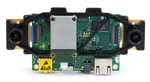
 Experiments were performed where the state estimation algorithm was tested with the VI sensor hardware. For comparison the pose trajectory was recorded using an indoor GPS solution. Multiple datasets covering slow and fast rotations and translations were recorded using the indoor GPS system rigidly attached to the VI sensor.
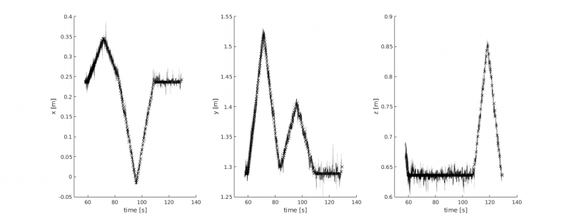
The constant transformation between the IGPS reference point and the IMU frame of the VI sensor was determined using a subset of the data. The choice was verified using a different dataset showing a difference of $5~cm$ in the worst case. The Figure to the right shows a qualitative comparison between the batch estimation and the recorded IGPS data. The estimated state trajectories consisting of 10 states each are drawn as transparent, overlapping lines while the IGPS data is represented by crosses. It is visible that previous estimates are improved in later iterations and that the first states in the trajectory are usually more accurate than the latest. The deviation from the IGPS dataset after transformation is approximately $2~cm$. It is to be expected that the precision of the target identification improves when moving closer to the target, because translational perturbations will then result in higher amplitudes in image space. The global coordinate system was chosen such that it aligns with the target, and the nominal distance between the camera and target was roughly $1~m$.
Experiments were performed where the state estimation algorithm was tested with the VI sensor hardware. For comparison the pose trajectory was recorded using an indoor GPS solution. Multiple datasets covering slow and fast rotations and translations were recorded using the indoor GPS system rigidly attached to the VI sensor.
The constant transformation between the IGPS reference point and the IMU frame of the VI sensor was determined using a subset of the data. The choice was verified using a different dataset showing a difference of $5~cm$ in the worst case. The Figure to the right shows a qualitative comparison between the batch estimation and the recorded IGPS data. The estimated state trajectories consisting of 10 states each are drawn as transparent, overlapping lines while the IGPS data is represented by crosses. It is visible that previous estimates are improved in later iterations and that the first states in the trajectory are usually more accurate than the latest. The deviation from the IGPS dataset after transformation is approximately $2~cm$. It is to be expected that the precision of the target identification improves when moving closer to the target, because translational perturbations will then result in higher amplitudes in image space. The global coordinate system was chosen such that it aligns with the target, and the nominal distance between the camera and target was roughly $1~m$.
 An advantage of sensor fusion is the ability to estimate the pose of the camera although the target has left its field-of-view.
However, the estimation now solely relies on the integration of IMU measurements which results in drifting state variables. In the example to the left, each position variable drifted by about $10~cm$ in $0.7$ seconds before target identification could be re-established. Longer interruptions cause a severe deviation of the real position (e.g. $50~cm$ in $3.2$ seconds). One of the sources of this behaviour is gyro noise which leads to an inaccurate estimation of the camera orientation. This orientation is used to remove the influence of the earth's gravity from the acceleration measurements. Other causes can be found in the simple Euler Forward integration pattern and irregularities of the filter update frequency.
An advantage of sensor fusion is the ability to estimate the pose of the camera although the target has left its field-of-view.
However, the estimation now solely relies on the integration of IMU measurements which results in drifting state variables. In the example to the left, each position variable drifted by about $10~cm$ in $0.7$ seconds before target identification could be re-established. Longer interruptions cause a severe deviation of the real position (e.g. $50~cm$ in $3.2$ seconds). One of the sources of this behaviour is gyro noise which leads to an inaccurate estimation of the camera orientation. This orientation is used to remove the influence of the earth's gravity from the acceleration measurements. Other causes can be found in the simple Euler Forward integration pattern and irregularities of the filter update frequency.
Overall, the computational performance of the state estimation algorithm is satisfying. Using a batch size of 10 plus one trailing state results in an average update frequency of about $50~Hz$. This corresponds to a trajectory length of $0.5$ seconds, assuming the target does not leave the field-of-view. Using a higher batch size results in a longer observable state trajectory at the expense of computational cost. When choosing a batch size higher than 14 the optimization is no longer able to keep up with the target identification. The optimization itself usually only requires between 1 and 3 steps, which stems from the fact that the cost functions are well-behaved and the starting position is usually already close to the minimum. Ceres solver reports that 95% of the time is spent in the linear solver stage which is hard to improve upon.
<latex> {\fontsize{12pt}\selectfont \textbf{Conclusions} </latex>
A general batch estimation framework has been built and tested, both in simulation and using the VI sensor. IMU and visual data have been fused to estimate a trajectory spanning $0.5$ seconds at $50~Hz$. Although the algorithm can handle a short loss of visual contact to the target, it diverges too quickly from the true pose.
The framework was designed to consist of an application-independent layer to solve a general batch estimation problem (which can be used for other projects as well) and an application-specific ROS node for the given task.
<latex> {\fontsize{12pt}\selectfont \textbf{Future Work} </latex>
- The estimator has no knowledge about the absolute position in the room, but only the relative pose from the end-effector to the target. Adding more sensors (such as base pose estimation or joint angles) to the batch estimation would increase the accuracy of the prediction, but also need more computational power.
- Determining system parameters such as the covariance matrices $P_0$, $Q_k$ and $R_k$ and how they should evolve over time has to be investigated. These parameters act as cost function weights and determine how the algorithm behaves.
- At the current stage an Euler Forward scheme is used for the integration of the IMU measurements. This could be replaced by a Tustin or Runge-Kutta scheme for better accuracy during phases where the target leaves the field-of-view of the cameras.
Page Tools
