LAB

<latex>{\fontsize{16pt}\selectfont \textbf{Unit Quaternion Parameterization for the iLQG Algorithm and Application to the In-Situ Fabricator}} </latex>

<latex>{\fontsize{12pt}\selectfont \textbf{[Lanke Fu]}} </latex>
<latex>{\fontsize{10pt}\selectfont \textit{[Semester Thesis]}} </latex>

<latex> {\fontsize{12pt}\selectfont \textbf{Abstract} </latex>

In-situ fabrication is a state of the art in the digital fabrication industry which focuses on automating construction tasks in unpredictable environments. The emphasis is not only on improving the efficiency of construction but also on generating new construction techniques to accommodate new designs in the architecture industry. At the ADRL, the In-Situ Fabricator (IF), a differentially driven robot, is being developed to automate construction tasks. To improve the efficiency of the control efforts with which IF manoeuvres through the work space, efforts are being put into generating control sequences online using the iLQG algorithm. This work contributes by introducing an orientation parameterization more suitable for the non-linear optimization carried out in the iLQG algorithm than the previously used Euler angle parameterization. The results are shown in simulation. Comparisons are made between the trajectories derived from this new parameterization and the former, Euler angle parameterization.

<latex> {\fontsize{12pt}\selectfont \textbf{Introduction} </latex>

<latex> {\fontsize{10pt}\selectfont \textbf{The In-Situ Fabricator} </latex>


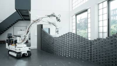
The IF is a research platform for developments in automated construction. The 6 degree of freedom robotic arm mounted to it is a model IRB 4600 industrial robotic arm from ABB with a 2.55m reach. Its relatively small size compared to the space available at a typical construction site, as well as the long reach of its arm enables the exploration of new construction designs. This is an improvement over more traditional approaches to digital fabrication where the size of the manipulator is typically larger than the design being formed.
The dynamical model of IF consists of 3 degrees of freedom in its base's orientation, 3 degrees of freedom in its base's position relative to the construction site reference frame and 6 degrees of freedom of its arm's joints. In this thesis, the simulation of the IF assumes a planar model in which the IF loses two degrees of freedom in rotation (only yaw about the vertical axis is maintained) and its translations are restricted to motions on the horizontal plane. Here on, the variable $x(\cdot)$ is used to denote the vector of these degrees of freedom along with their first-order derivatives. In actuation, the IF has 8 degrees of freedom. Its 6-jointed arm is commanded by torque input $[N\cdot{} m]$ and a force input [N] commands the two tracks driving its base. Here on, the variable $u(\cdot)$ is used to denote the vector of these inputs.

<latex> {\fontsize{10pt}\selectfont \textbf{The iLQG Algorithm} </latex>

In the task of calculating efficient control inputs for driving IF to a desired state at a certain terminal time, the following equation is used to quantify the sum of the control effort spent and the penalty on deviation between the desired state and the actual state of the robot.

$$ J = \mathit{h}(x_{final}) + {\sum_{t=0}^{t_{final}}}g(t,x(t),u(t)) $$ This discrete time formulation quantifies the task cost in two ways. Firstly, the function $h(\cdot)$ is possibly a non-linear function which penalizes the deviation of the final state of the robot from the desired final state. Secondly, the function $g(\cdot)$ penalizes the control effort and state deviation at every time step, from some nominal control and state reference for that time step. As will be shown later, the definition of the function $g(\cdot)$ can be used to generate via-point states so that the robot visits a particular state at the via-point time, before arriving at the final state. While the optimal control trajectory for the cost shown in (1) could be computed by solving the associated Hamilton-Jacobi Bellman equation, the problem is generally intractable for systems exhibiting non-linear dynamics and cost functions. The iLQG algorithm ¹⁾ presents a sub-optimal solution to the problem but is effective in computing such solutions efficiently with fast convergence properties as described in ²⁾.

This iterative algorithm is initialized with a stabilizing control sequence, to maintain its initial state. In this case this is generated using a Linear Quadratic Regulator (LQR). Improvement over succeeding iterations is achieved by adding to this stabilizing control sequence a feed-forward term. This feed-forward term, for each time-step, is calculated by generating an LQR with the system's linearized dynamics at the current time step and its associated cost-to-go function. The cost-to-go function is representative of the cost that would be accumulated to get from the current state and time step, to the desired final state at terminal time. In the current simulation pipeline, the linearized dynamics of the system are calculated using a perturbation scheme. Let $f(\cdot)$
define the system's dynamics where $$ \frac{d}{dt}x(t) = f(x(t),u(t),t) $$ Then to a first-order approximation, the dynamics of the perturbations about a nominal state $\=x$ and control input $\=u$ is given by $$ \frac{d}{dt}\delta x(t) = \frac{\partial f}{\partial x}|{_{\={x},\={u}}} \delta x(t) + \frac{\partial f}{\partial u}|{_{\={x},\={u}}} \delta u(t) $$ For $x \in \mathbb{R}^N$ let the matrix $A \in \mathbb{R}^{N \times N}$ represent the matrix of the partial derivatives $ A = \left[ \begin{array}{ccc} \frac{\partial f_1}{\partial x_1} & \dots & \frac{\partial f_1}{\partial x_N}
\vdots&\ddots&\vdots
\frac{\partial f_N}{\partial x_1} & \dots & \frac{\partial f_N}{\partial x_N}

\end{array} \right] $ . The perturbation scheme mentioned here obtains the $i$-th column of $A$ by applying a minor perturbation $\epsilon$ to the state $x_i$ and obtaining the difference in the function $f$, between the nominal and the perturbed state, $\delta f$ . From this, a linear approximation to the partial wrt state $x_i$ can be obtained through the quotient $\frac{\delta f}{\epsilon}$. This is done while all other states apart from $x_i$ are held constant. This procedure is mentioned here because it has an effect on the choice of orientation parameterization, as will be discussed later.

<latex> {\fontsize{10pt}\selectfont \textbf{The Pre-existing Caveat} </latex>

In the video above IF is commanded to traverse from the initial state $x(0)=[0,0,0,0,0,0.5,0,-0.8,0.8,0,\dots,0]^T$ (from here on referred to as trim state) to the final state $x_{final}=[0,0,2\pi,0,0,0.5,0,-0.8,0.8,0,\dots,0]^T$. In the vector $x(\cdot)$ the first three components are the orientation of IF relative to the construction space reference frame, in the Euler angle XYZ formulation. The following three components represent its center of mass position and the remaining six components are the deflection angles of its arm's joints. As seen in the video, the robot rotates a full cycle in the counter-clockwise direction, even though the underlying pose represented by a yaw of $0$ $radian$ is equivalent to a yaw of $2\pi$ $radians$.
The example demonstrates a caveat of parameterizing the IF's orientation using the Euler angle formulation. The cost function used for the iLQG algorithm penalizes quadratic approximations to the Euclidean distance between a desired robot state and its actual state, at a given time step. Therefore, in the example above, the algorithm converges in a control sequence that redundantly manoeuvres the robot in order to minimize the penalty incurred from the Euclidean difference between the initial and final state - reluctant of the actual orientations represented.

<latex> {\fontsize{10pt}\selectfont \textbf{Quaternions} </latex>
Unit quaternions in representing rotation sequences, are advantageous due to their capability to encode the shortest rotation. Suppose a unit quaternion $$ \mathbf{q_{BI}} = \left[ \begin{array}{c} q_0
q_1 \hat{\mathbf{i}}
q_2 \hat{\mathbf{j}}
q_3 \hat{\mathbf{k}}\end{array} \right]

=

\left[ \begin{array}{c} \cos{\frac{\alpha}{2}}
\sin{\frac{\alpha}{2}a}

\end{array} \right] $$ represents the orientation of IF's body frame $B$ with respect to(wrt) the construction site reference frame $I$. Intuitively, the orientation of the frame $B$ wrt $I$ can be visualized as rotating about an axis $a$ in the $I$ frame by an angle $\alpha$. Where the variables $a$ and $\alpha$ are as given by the equation above. Physically, a rotation of $\alpha$ about an axis $a$ is the same as rotating by an angle $2\pi-\theta$ about this same axis. Therefore, through the above equation it is evident that a quaternion $\mathbf{q}$ and its negative counterpart $-\mathbf{q}$ represent the same orientation. However, as previously mentioned, these two quaternions represent different rotation sequences where the shorter rotation sequence is represented by the quaternion with real part, $q_0<0$. With this criterion it is possible to determine the shortest rotation sequence between an initial and desired final orientation.
The composition of rotation sequences is equivalent to the multiplication of their corresponding quaternions. This multiplication is carried out as follows

$$ \mathbf{q}\otimes\mathbf{p} = \mathbf{M}_l(\mathbf{q})\mathbf{p} $$

Where the matrix $\mathbf{M}_l(\mathbf{q})$ according to the Hamilton convention is defined as

$$ \mathbf{M}_l(\mathbf{q}) = \left[\begin{array}{cccc} q_0 & -q_1 & -q_2 & -q_3
q_1 & q_0 & -q_3 & q_2
q_2 & q_3 & q_0 & -q_1
q_3 & -q_2 & q_1 & q_0 \end{array} \right] $$

The difference between the initial orientation $\mathbf{q}_0$ and the desired final orientation $\mathbf{q}_{final}$ is described by the quaternion error $q_{error}$ given by $$ \mathbf{q}_{error} = \mathbf{q}_{final}\otimes\mathbf{q}^{-1}_0 $$ where $\mathbf{q}^{-1}_0$ denotes the inverse of $\mathbf{q}_0$ and can be calculated through $$ \mathbf{q}^{-1} = \frac{\check{\mathbf{q}}}{||\mathbf{q}||} $$ and $\check{\mathbf{q}}$ is the quaternion conjugate given by $$ \check{\mathbf{q}} = \left( \begin{array}{c} q_0
-q_1 \hat{\mathbf{i}}
-q_2 \hat{\mathbf{j}}
-q_3 \hat{\mathbf{k}}\end{array} \right) $$

<latex> {\fontsize{12pt}\selectfont \textbf{Implementation} </latex>
In this section, a 3-parameterization derived from the quaternion representation of the orientation of a rigid body is described. It's application in the iLQG algorithm follows.
In what has been presented so far, a technique for representing the shortest rotation sequence between two orientations using quaternions is discussed. To proceed with the implementation of the iLQG algorithm, however, a further step has to be taken due to a practical limitation. Namely, the perturbation scheme mentioned above which is used to retrieve the system's linearized dynamics cannot be applied to unit quaternions directly. In perturbing any of the quaternion's four dimensions, the unit norm property is violated. As a result, the properties of a unit quaternion is describing orientations will no longer hold.

This motivates the creation of parameterization technique which benefits from the quaternion property of representing shortest rotation sequences while at the same time, is suitable for the linearization scheme mentioned above. In ³⁾ a technique is presented which generates a 3-dimensional orthogonal basis at a given nominal quaternion state. Using this basis, 3 parameters are sufficient to describe any other orientation relative to this nominal state.

Here, a similar approach will be taken to use 3 parameters to parameterize the shortest geodesic arc between the initial and desired final orientation. In the simulation pipeline based in the Robot Operating System (ROS) is first converted from Euler angles XYZ formulation to unit quaternions using the Kindr package. Next, a new reference frame is created in which the initial state of the robot becomes the new reference frame origin and the desired final orientation of the robot is represented by the quaternion error (described earlier). Using a technique similar 3), 3 parameters are used to parameterize orientations relative to the initial state of the robot. The transformation from the quaternion error $\mathbf{q}$ (desired final state) to the 3-parameter error vector $v_{error}$, with the identity quaternion(reference frame origin) as the operating point is given as follows: $$ v_{error} = 2\arccos(q_{error_0})\frac{\mathbf{imag}(\mathbf{q}_{error})}{|\mathbf{imag}(\mathbf{q}_{error})|} $$
Where $q_{error_0}$ is the real part of the error quaternion and $\mathbf{imag}(\mathbf{q}_{error})$ is the imaginary part of the quaternion error.

Due to its ease of intuition, it might be beneficial to convert the 3-parameters back into Euler angles. To do so, a given 3-parameter representation $v$ is first transformed into a quaternion representing the orientation in the new reference frame through, $$ \mathbf{q_bi = \left[ \begin{array}{c} \cos{\frac{ {\left| \left| v \right | \right |} }{2}}
\sin{\frac{ {\left| \left| v \right | \right |} }{2}} \cdot \frac{v}{ {\left| \left| v \right | \right |} }

\end{array} \right] $$ Since the reference frame was changed to the initial orientation of the robot during the 3-parameterization, to obtain the pose represented by $v$ in the original coordinate frame $\mathbf{q}_{BI}$ a quaternion multiplication with the initial quaternion state is necessary i.e. $\mathbf{q_{BI}} = \mathbf{q_bi_initial}} \cdot \mathbf{q_bi $. From $\mathbf{q_{BI}}$ the desired Euler angle parameterization can be obtained using the equations shown in ⁴⁾.

<latex> {\fontsize{12pt}\selectfont \textbf{Results} </latex>

The 3-parameterization technique is put to test for the simulation of IF. As seen in the introduction section, the previously used Euler angle formulation was not able to depict the shortest rotation sequence for certain setups. The example seen on the left is one of such cases. The left-most image shows the desired final pose of IF, whereas the middle image shows its initial pose.

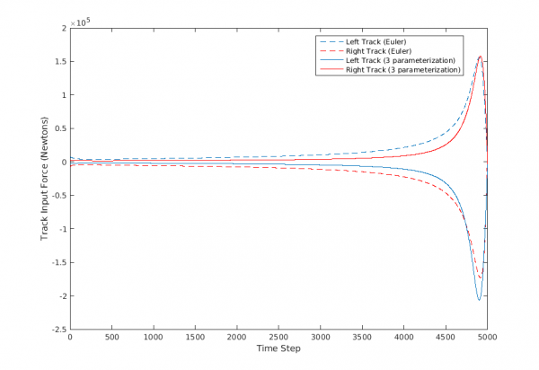
Below, the resultant trajectories calculated from the two different parameterization techniques are shown in the form of output forces from the two driving tracks of IF.

The IF starts this task from rest and its joint states both at the initial and desired final state are at trim. Reasonably, an efficient manoeuvre would turn counter-clockwise towards the final state. As seen from the track input plot on the left, the Euler angle formulation resulted in a clock-wise turn (left track inputs are positive), unlike the 3-parameterization which resulted in a counter-clockwise turn.

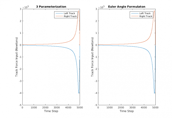
The task shown on the left serves to verify the validity of the 3-parameterization, using a scenario in which the Euler parameterization calculates an intuitively efficient path. The IF is commanded to manoeuvre from an initial yaw orientation of $0$ $radian$ to $\pi$ $radians$. Below are the results.

As seen above, in such a scenario where the Euler parameterization was capable to arrive at the efficient rotation sequence, the output track inputs in both paramterizations are identical.

<latex> {\fontsize{12pt}\selectfont \textbf{Conclusion} </latex>

The current technique maintains the input of task parameters defining the orientation of IF’s base in Euler angles. Through a transformation using the 3 parameterization technique presented, it is able to calculate the shorter rotation sequence which was not always the case for the Euler angle formulation. The results for paths mutually feasible in the two parameterization techniques were simulated and the 3 parameterization’s results agree with those from the Euler formulation. More complex tasks can be achieved by incorporating one via-point, in which case the reference origin is transformed to the pose of the robot at the via-point state. This way, the algorithm calculates the shortest sequence between the initial state and the via-point state as well as from the via-point state to the final state.

<latex> {\fontsize{12pt}\selectfont \textbf{Future Works} </latex>

• Creating adaptive state-deviation cost matrices, to utilize this parameterization technique in non-planar scenarios.
• Investigation into incorporating more than one via-point.