LAB

<latex>{\fontsize{16pt}\selectfont \textbf{Learning rigid body dynamics of}} </latex>
<latex>{\fontsize{16pt}\selectfont \textbf{constained multibody systems}} </latex>

<latex>{\fontsize{12pt}\selectfont \textbf{Ruben Grandia}} </latex>
<latex>{\fontsize{10pt}\selectfont \textit{Master thesis, RSC}} </latex>

<latex> {\fontsize{12pt}\selectfont \textbf{Abstract} </latex>

Model based control techniques show promising results in simulation, but often face degraded performance when deployed on hardware. Since these methods heavily rely on the correctness of the model, this performance loss can be ascribed to model mismatch. In order to reclaim this loss in performance it is proposed to learn a better model from data.This idea is pursued in the context of HyQ, a hydraulically-actuated quadruped robot.

While there are many ways to obtain a better model, it is proposed to learn a force error term between observed data and the inverse dynamics of the nominal model. This additive formulation results in a local dependency on the learning method and in this sense provides robustness against situations where the robot is far away from the space explored in the training data.

The inevitable existence of contact forces in legged robots complicates the model learning. Because reliable estimates for the contact forces are challenging to obtain, the proposed method projects the dynamics into the null space of the constraints. As a main contribution, this work proposes a change of basis hereafter to construct a formulation in the constraint consistent subspace that generalizes the learned model over all possible constraint configurations.

A series of standing and walking trajectories are performed to collect the necessary data for model learning. In order to capture a wide range of the dynamics, a method is proposed to generate random trajectories in the coordinates of the floating base. A controller to track these reference trajectories is designed as well.

Locally Weighted Projection Regression (LWPR) and Gaussian Process Regression (GPR) are explored as general function fitting techniques to learn the force error model as a function of the generalized coordinates, velocities, and accelerations. Both methods are shown to result in more accurate model predictions. Where LWPR has the advantage in terms of computational complexity, GPR is able to obtain similar performance with much less data.

A model based inverse dynamics method that simultaneously optimizes input torques and contact forces is extended to incorporate the learned model. Experiments on hardware show that using a learned model results in significantly less feedback torque and better joint angle tracking when compared to the same controller using the nominal model.

<latex> {\fontsize{12pt}\selectfont \textbf{Projected error model formulation} </latex>

The desire to be robust against configuration far away from training samples motives the approach of adding a machine learning term to the already existing nominal RBD model. This approach showed promising results in a exploratory semester project for the case of quadrotors ¹⁾. Adding the error term as a generalized force was selected over an acceleration based formulation after comparison. The nominal RBD augemented with the force error model is then given by

\begin{equation*} \matr{M} \ddvect{q} + \vect{h}= \matr{S}^T \vect{\tau} + \matr{J}_c^T \vect{\lambda} + \vect{\Phi}\left(q, \dot{q}, \ddot{q}\right) \end{equation*}

Since the contact forces $\vect{\lambda}$ are not used in this work, the dynamics are projected to the constraint consistent subspace ²⁾. Here, the projected error model can be observed from data with

\begin{equation*} \matr{P} \vect{\Phi} = \matr{P} \left(\matr{M} \ddvect{q} + \vect{h} - \matr{S}^T \vect{\tau} \right) \end{equation*}

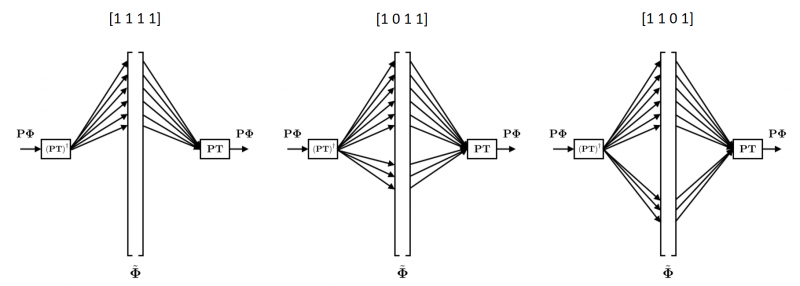
It was observed that the projected error model would change per foothold, so a contact independent formulation was derived. The observable part of the transformed space can be uniquely computed from

\begin{equation*} \left[ \begin{array}{l} \tilde{\vect{\Phi}}_0
\tilde{\vect{\Phi}}_{u} \end{array} \right] = \begin{bmatrix} \matr{J}^T_0, \matr{P}\matr{J}^T_{u} \end{bmatrix}^{\dagger} \matr{P}\vect{\Phi} \end{equation*}

Finally, when predictions are to be made, the transformation back to the projected generalized force space can be made with

\begin{equation*} \matr{P}\vect{\Phi} = \matr{P} \matr{T} \tilde{\vect{\Phi}} \end{equation*}

The procedure of mapping the error model into the transformed space, selecting the right elements, and mapping them back is visualized in the following figure.

In conclusion, the model learning in this formulation boils down to learning the vector function $\tilde{\vect{\Phi}}\left(\vect{q}, \dvect{q}, \ddvect{q}\right) \in \mathbb{R}^{n+6}$ from data $\{\text{fic}, q, \dot{q}, \ddot{q}, \vect{\tau} \}$, where $\text{fic}$ contains the foothold of the sample.

<latex> {\fontsize{12pt}\selectfont \textbf{Supervised error model learning} </latex>

The current section covers the machine learning methods and procedures that enable the learning of the targeted functions. To highlight the fact that the problem is a general function approximation problem, the function to be learned is repeated alongside the supervised learning notation. The multivariate function $\vect{f}(\vect{x})$ is learned elementwise and the goal is thus to learn $n+6$ functions $y_i = f_i(\vect{x})$ from samples $\{\vect{x}, \vect{y}\}$.

\begin{equation*} \label{eq:lea:phi_tilde_goal} \tilde{\vect{\Phi}}\left(\vect{q}, \dvect{q}, \ddvect{q}\right) & = \begin{bmatrix} \matr{J}^T_0, \matr{P}\matr{J}^T_{/c} \end{bmatrix}^{\dagger} \matr{P} \left(\matr{M} \ddvect{q} + \vect{h} - \matr{S}^T \vect{\tau} \right) \end{equation*}

\begin{equation*} \vect{f}(\vect{x}) & = \vect{y} \end{equation*}

Where $\vect{x} \in \mathbb{R}^{3(n+6)-4}$ is the input space $[\vect{q}^T, \dvect{q}^T, \ddvect{q}^T]^T$ after removing the yaw and base positions $[\psi, x, y, z]$. These states are removed because they have an arbitrary value depending on the state estimator initialization and do not affect the system dynamics. For the case of HyQ the input and output dimensionality are $3(n+6)-4 = 50$ and $n+6 = 18$ respectively.

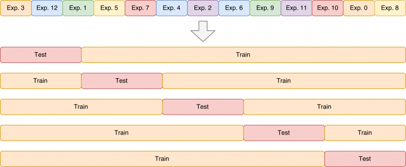
Two different methods for supervised learning are applied in this work; Locally weighted projection regression (LWPR) ³⁾, and Gaussian process regression (GPR) ⁴⁾. Both methods are tuned using crossvalidation. However, because the data is temporally correlated, special care should be taken in setting up the cross validation. First, all experiments are concatenated in random order. A 5-fold crossvalidation is then performed by splitting blocks of data. This procedure is illustrated in the figure below.

To compare the performance of the used methods, a metric is used that relates to the initial problem of interest, i.e. model learning. The estimate of the transformed projected error $\widehat{\tilde{\vect{\Phi}}}$ is taken back to the generalized force space in order to compute the estimated projected error $\widehat{\matr{P} \vect{\Phi}}$. The nMSE performance is then computed by comparing the estimated dynamics and projected inputs via the equation below, which provides an nMSE measure in each of the 18 DoFs.

\begin{equation*} nMSE = \frac{1}{N \cdot \mathbb{V}(\matr{P} \matr{S}^T \vect{\tau}) } \sum_{\{\text{fic}, \vect{q}, \dvect{q}, \ddvect{q}, \vect{\tau} \}} (\matr{P} \vect{\Phi} - \widehat{\matr{P} \vect{\Phi}})^2 \end{equation*}

This shows how the model learning performance is measured by the mean squared error in predicting the projected error and normalizing with the variance of the projected inputs. The performance of the nominal RBD model is found by setting $\widehat{\matr{P} \vect{\Phi}}$ to zero.

This nMSE performance metric is computed for different motions and trajectories of which the data has not been used for model training or parameter tuning. The results on standing trajectories are

For walking motions two type of experiments are performed. One where the same reference trajectory was already used in one of the training experiments, and one where the reference trajectory is new but similar to the walks used for training. The results are plotted below first for the seen walks and then for the unseen walks.

In general the learned models outperform the nominal model. The difference between the seen and unseen walk indicate that model performance degrades for data from novel trajectories and therefore potentially for new parts of the input space. While the nMSE values cannot be directly compared because of the different normalizations depending on the experiments, the comparison with the nominal model suggest that the learning gives less of an improvement.

<latex> {\fontsize{12pt}\selectfont \textbf{Applications in control} </latex>

An existing model based optimal control method is extended to incorporate the learned model and implemented on hardware to test the performance of model based control methods with learned models. The HyQ legged robot is used as the system and the resulting trajectories from the direct collocation framework in ⁵⁾ are used the reference trajectory.

The feedforward part of the controller is based on inverse dynamics control with optimal distribution of contact forces ⁶⁾. This controller defines a quadratic program (QP) and uses a trick related to the projection trick to split the dynamics in an unconstrained and constrained part. The QR decomposition of the constraint Jacobian is given by

\begin{equation*} \matr{J}_c^T = \begin{bmatrix} \matr{Q}_c, \matr{Q}_u \end{bmatrix} \begin{bmatrix} \matr{R}
\matr{0} \end{bmatrix} \end{equation*}

The QP formulation is then extended to use the learned model:

\begin{equation*}

\begin{array}{rrcl}

\multicolumn{4}{c}{\underset{\tau}{\text{min}} \quad \frac{1}{2} \vect{\tau}^T \matr{W}_{\vect{\tau}} \vect{\tau} + \vect{b}_{\vect{\tau}}^T \vect{\tau} + \frac{1}{2} \vect{\lambda}^T \matr{W}_{\vect{\lambda}} \vect{\lambda} + \vect{b}_{\vect{\lambda}}^T \vect{\lambda} } \\ \\

\textrm{s.t.} & \matr{Q}_u^T\matr{S}^T \vect{\tau} & = & \matr{Q}_u^T\left(\matr{M} \ddvect{q}^d + \vect{h} \right) - \color{red}{\matr{Q}_u^T \matr{P} \vect{\Phi}}
& \matr{C}_{\vect{\tau}} \vect{\tau} &\leq& \vect{d}_{\vect{\tau}}
& \matr{C}_{\vect{\lambda}} \vect{\lambda} &\leq& \vect{d}_{\vect{\lambda}}
\end{array} \end{equation*}

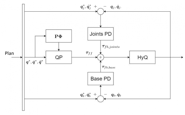
The figure above shows the resulting control diagram after inserting the feedforward QP controller defined in the previous section. For the feedback part a seperate stabilization for the joints and the base coordinates is used. These feedback controllers are identical for all experiments. Because the planned trajectory is known in advance, the feedforward terms $\vect{\tau}_{ff}$ can be computed offline. This strategy was adopted when using both LWPR and GPR as the learned model. Also a version that adapt the learned model of LWPR online is tested.

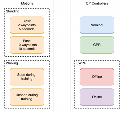
The following sections present the results of hardware experiments under various motions defined in and variations of the QP controller. An overview of all considered variations is shown below.

An impression of both type standing and walking of motions is provided below.

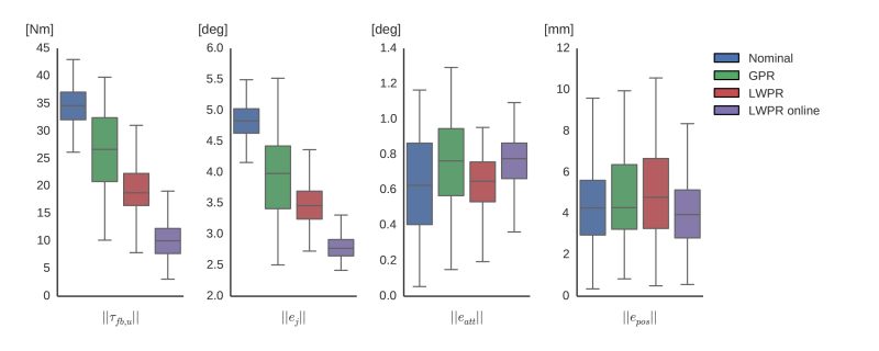
The performance of the QP controller under the four different models is shown for the fast trajectory hereafter. For both slow and fast trajectories the learned models outperform the nominal model on the applied unconstrained feedback $\|\vect{\tau}_{fb,u}\|$ and joint tracking performance. The performance improvement is larger for the slow trajectory, which indicates that these static type of errors are learned more easily. Also, on the fast trajectory the online adaptation is seen to have a great benefit. In the tracking of the base coordinates little improvement is seen. However, looking at the scale of the errors, the errors are already low in general.

For the walking trajectories both a reference that was used for generating training sample, the seen walk, and a new but similar walking trajectory, the unseen walk, are considered. The results for the seen walk are shown below.

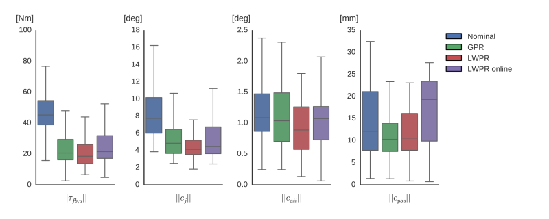
Again, the learned models outperform the nominal model and the average unconstrained feedback torque is more than halved for the seen walk. The performance difference on the unseen walk is slightly less, but still significant. This shows that the learned model is able to generalize beyond the exact trajectories it was trained on. Similar to the standing trajectory, the base tracking performance does not benefit from the learned model.

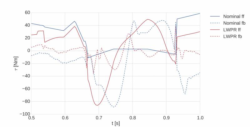
A closer look at the torques in the knee joint during the leg swing phase is given in the following figure. Where the nominal model almost completely relies on feedback, the LWPR model is able to provide a feedforward signals that allows for a low feedback. Moreover, the inherent delay of relying on feedback becomes apparent. The nominal model has to wait for an error to build up before the feedback torques become active, while the learned model applies the correct torque right away. This results in a major reduction of the upper extremes of the joint error distributions in the boxplots for walking.

<latex> {\fontsize{12pt}\selectfont \textbf{Conclusion} </latex>

With the objective of recovering the observed performance loss of model based control techniques when implemented on hardware, it was proposed to learn a better model in order to reclaim performance of these type of methods on the real robot.

Starting from the introduction of a force error term between the existing rigid body dynamic and observed data, the main contribution of this work is the formulation of the projected error learning in a space that is invariant to the contact configuration. It was shown that using locally weighted projection regression (LWPR) and Gaussian process regression (GPR) as general function learning methods in that space provides more accurate model predictions for both standing and walking trajectories. Comparing the computational complexity of both methods it can be concluded that LWPR has a clear edge over GPR both in terms a training time and time to prediction. However, GPR does attain a similar prediction performance from significantly less data and could therefore be the preferred method in applications where computation is not an active constraint.

When using the learned models in a feedforward strategy that optimizes the input torques while simultaneously taking into account the contact force constraints, a significant performance improvement on the HyQ robot was shown. The required feedback effort is approximately halved and tracking of the joint coordinates is improved by the same factor. Moreover, the leg swing during walking is driven by the feedforward signal under the learned model, where the controller that uses the nominal model relies completely on feedback.

In conclusion it was shown that (1) error learning results in a more accurate model, and that (2) using this model in a model based framework significantly improves performance on hardware. This confirmation of the posed hypothesis opens the door to more complex motions that are currently infeasible for model based control methods under the standard model. Moreover, the promising results of online learning could allow a robot to continuously adapt to model changes originating from minor damage or a change of payload for example.

<latex> {\fontsize{12pt}\selectfont \textbf{Future Work} </latex>

With the current implementation as a starting point, the most direct way of improvement would be the addition of more data from a more diverse set of motions. The fact that the online learning managed to quickly outperform the offline version of the same algorithm on a standing trajectory suggests that there is more to learn about the model than currently contained in the training data.

Afterwards, it is to be shown that the learned model now allows for motions that were infeasible before. All current experiments were already possible under the nominal model, be it with less performance. The challenge here is the need to obtain training data that generalizes to these motions. The similar performance obtained on an unseen walk in this work is promising, but the extent to which the learned models generalize is in general still an open question.

The unsuccessful attempt to use the model for feedback linearization is briefly discussed in the thesis report. Pursuing this direction gives rise to fundamental questions of stability and robustness of using a learned model for control. The current assessment is that by treating the learning of a model and the model based control as separate problems, some key properties are missed that prevent the successful combination of the two. The learning method for example does not care about the local properties of the model, while feedback linearization relies on the model to be at least invertible.