LAB

<latex>{\fontsize{16pt}\selectfont \textbf{Human-Robot Interaction Force Estimation for Transparency Control on Wearable Robots}} </latex>

<latex>{\fontsize{12pt}\selectfont \textbf{[Lisa Hammer]}} </latex>
<latex>{\fontsize{10pt}\selectfont \textit{[Master Project ME]}} </latex>

<latex> {\fontsize{12pt}\selectfont \textbf{Abstract} </latex>

Within recent years, exoskeleton robots have become a widely popular research topic in robotics and rehabilitation engineering, enabling both healthy and disabled users to perform tasks they would otherwise not be capable of. The EU Balance Project, which this thesis was a part of, is an exoskeleton project aiming at developing a supporting robot for postural balance. For this, the exoskeleton should support and guide the user whenever a balance problem like stumbling occurs but be imperceptible otherwise. This concept of being imperceptible to the user is called transparency in human-robot interaction. It requires the robot to compensate for all joint forces like friction or damping and follow the human movement exactly.
This project aimed at simulating a novel transparency control paradigm ¹⁾ and implementing it on a linear test bench. The focus specifically lay on estimating the interaction force between the robot and the human, which in real world applications can be difficult to measure directly. We used an acceleration feedforward and feedback controller as well as a force feedback controller to reduce the interaction force to zero. The interaction force used by the force controller was estimated with a Kalman filter.
We simulated this system in MATLAB and evaluated controller and Kalman filter performance. We then adjusted our linear test bench to obtain the best possible controller performance. Finally, we ran first experiments on the setup to prove the real-life viability of our approach.

<latex> {\fontsize{12pt}\selectfont \textbf{System Model} </latex>

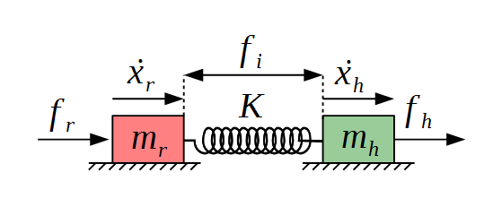
The left figure shows the linear model we used for simulation and our linear test bench. It consists of two masses which are connected by a spring. The masses represent the robot and the human limb, the spring corresponds to the elastic attachment between the exoskeleton and the human body. With this model, the linear system dynamics become

<latex>{\begin{equation*} \dot{f}_i&=K(\dot{x}_r-\dot{x}_h) \end{equation*}</latex>

for the spring,

<latex>{\begin{equation*} f_r-f_i&=m_r\ddot{x}_r \end{equation*}</latex>

for the robot, and

<latex>{\begin{equation*} f_h+f_i&=m_h\ddot{x}_h \end{equation*}</latex>

for the human, leading to

<latex>{\begin{equation*} m_r\ddot{f}_i+f_i K = K(f_r-m_r\ddot{x}_h) \end{equation*}</latex>

as the combined interaction force dynamics.

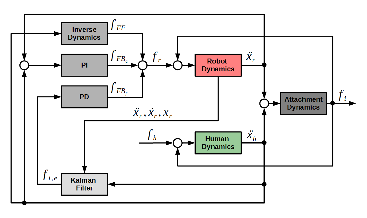
These dynamic equations correspond to the right part of the controller block diagram above, describing the uncontrolled system behaviour of the robot, the human and the attachment. In the left part of the block diagram we see the three controllers and the Kalman filter. Hereby, the first controller is a simple acceleration feedforward controller of the form

<latex>{\begin{equation*} f_{FF} = m_r \ddot{x}_h \end{equation*}</latex>

The two other controllers are a PI and PD controller on acceleration and force respectively, described by the following equations.

<latex>{\begin{equation*} f_{FB,a}=K_{p,a}(\ddot{x}_h-\ddot{x}_r)+K_{i,a}(\dot{x}_h-\dot{x}_r) \end{equation*}</latex>

<latex>{\begin{equation*} f_{FB,f}= -K_{p,f} f_i - K_{d,f}\dot{f}_i \end{equation*}</latex>

Integrating those controllers into the system dynamics in place of the robot force $f_r$ leaves us with

<latex>{\begin{equation*} m_r\ddot{f}_i+f_i K & = K(K_{p,a}(\ddot{x}_h-\ddot{x}_r)+K_{i,a}(\dot{x}_h-\dot{x}_r) -K_{p,f} f_i - K_{d,f}\dot{f}_i) \end{equation*}</latex>

---

The Kalman filter consists of two stages, the prediction and the correction stage. In the prediction stage, the system state for the next time step is predicted according to a state-space model of the system. Additionally, the error covariance matrix P is predicted.

<latex>{\begin{equation*} x_{k}&=Ax_{k-1}+Bu_{k-1} \end{equation*}</latex> (predicting state)

<latex>{\begin{equation*} P_{k}&=AP_{k-1}A^T+Q \end{equation*}</latex> (predicting error covariance)

Hereby A and B are the state-space matrices, x is the state, and u the control input. Q is the process covariance matrix describing the uncertainty in the model used for prediction. The main part of the correction stage is the computation of the Kalman gain K, which is a correction factor to adjust the predicted state according to the current measurements. With this gain, the state and error covariance values are then corrected and the next prediction stage starts.

<latex>{\begin{equation*} K_k&=P_kH^T(HP_kH^T+R)^{-1} \end{equation*}</latex> (determining Kalman gain)

<latex>{\begin{equation*} x_k&=x_k+K_k(y_k-Hx_k) \end{equation*}</latex> (correcting state)

<latex>{\begin{equation*} P_k&=(I-K_kH)P_k &\tex \end{equation*}</latex> (correcting error covariance)

R is a measurement covariance matrix similar to the process covariance matrix in the prediction step, describing the uncertainty in the measurements y. I corresponds to the identity matrix and H is the measurement matrix describing the relation between x and y. We used human and robot position and velocity as our four states as well as measurements. From our estimated states we then computed the interaction force estimate with the dynamic equations shown in the previous section.

<latex> {\fontsize{12pt}\selectfont \textbf{Simulation} </latex>

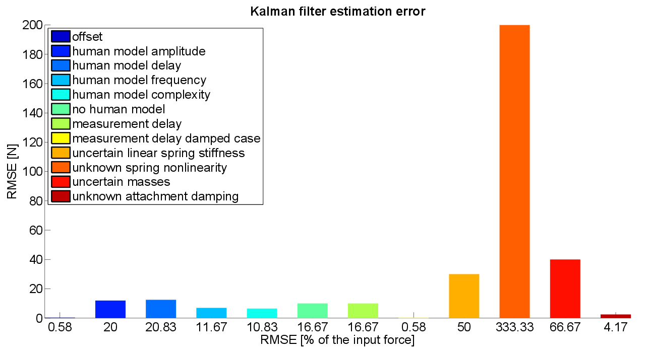
For simulation, we implemented the controllers and system dynamics shown above in MATLAB Simulink and simulated the model under different conditions. First, we evaluated the Kalman filter performance in terms of the root mean square error (RMSE) of the estimate. We varied certain parameters in either the model used for estimation or the system dynamics while leaving the respective other constant. All tested cases are listed in the figure on the bottom left. The values shown are a mean value of the RMSE for each case, since we performed several similar experiments for some situations. We can see that the most influential factor for accurate interaction force estimation by far is precise knowledge of the attachment dynamics. This becomes especially apparent when the spring is nonlinear. This is reasonable behaviour considering that the traditional Kalman filter, which we use, is a linear estimator and cannot account for nonlinear dynamics. While the remaining cases seem negligible next to the large influence of the attachment dynamics, issues like uncertain masses or delays and amplifications in our human model might become relevant depending on the hardware or estimator chosen and should be kept in mind.

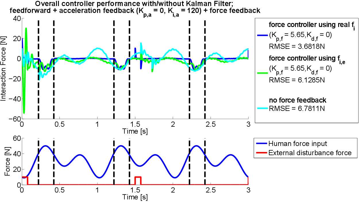
For controller evaluation we tuned our two feedback controllers so that, for every case, the phase margin was around 70°, the settling and rise times lower than 0.5s and 0.1s respectively and the overshoot smaller than 15%. Again, we performed different simulation experiments, varying e.g. actuator saturation, bandwidth or measurement delay. The overall controller performance is shown in the figure on the bottom right. In this case we used a small measurement delay of 1ms, 0.1\% measurement noise and fed the Kalman estimated interaction force into the force controller. In the bottom plot we see the human input force in blue, for which we used a sum of sines simulating a realistic human joint movement. In red we see an external pulse disturbance force leading to sharp peaks in the controlled force. The black lines represent the points where actuator saturation at 600N is entered and left. This occurs every time the human force reaches its higher peak. Within that interval, not even the 'ideal case' controller, which has exact information on the interaction force, can reduce it to zero since the actuator is unable to produce the required force. In green, we see the controller with the Kalman filtered interaction force. It cannot control fast force changes without starting to oscillate at a high frequency. This is due to the fact that the Kalman filter cannot estimate these fast, nonlinear changes accurately and thus the controller does not have the correct force information necessary to calculate the required control action. Apart from those highly oscillatory parts, this controller works reasonably well and keeps the interaction force close to zero. To have something to compare this case to, we performed the same experiment without any force controller whatsoever. We can see that, while the fast oscillations at the start are removed, the overall oscillation with the human input force increases significantly. This also shows in the control RMSE, which is slightly higher than for the case with a force controller. We thus conclude that a force controller can help overall controller performance unless the force dynamics are highly nonlinear.

<latex> {\fontsize{12pt}\selectfont \textbf{Hardware} </latex>
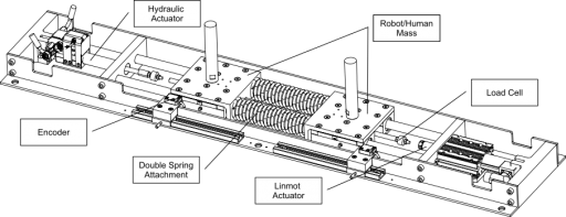
To be able to verify our simulation results on hardware, we adjusted an existing test setup (FC2D - Force Control in Two Degrees) to our needs. Firstly, we exchanged the microcontroller for a higher bandwidth version, enabling us to sample at 5kHz and thus giving us enough range to vary sampling frequencies while still retaining a stable controller. For this replacement we also had to adjust the remaining electronics to the new microcontroller voltage. Additionally, we replaced the previously used hydraulic actuators with higher bandwidth electric motors. This resulted in an overall much faster setup, which was critical for good force control performance. The following figure shows the setup with one electric and one hydraulic actuator. In addition to the shown components, each mass can be equipped with an IMU to measure acceleration.

<latex> {\fontsize{12pt}\selectfont \textbf{Experiments} </latex>
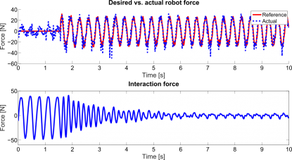
First, we performed a control experiment. Due to time constraints, it was only conducted with the feedforward controller. The following figure shows the results from this experiment. On the bottom we see the interaction force, on the top the control force input vs. the actual applied force. The controller is switched on at 1.5s. The feedforward controller brings the overall oscillations from the human input down to zero with a certain gradient between 1.5s and 6s. Then the only forces remaining in the system are oscillations stemming from the attachment dynamics, which the feedforward controller cannot compensate for. Force tracking works almost perfectly however, which leaves us optimistic that these forces will be compensated for by the feedback controllers once they are implemented. 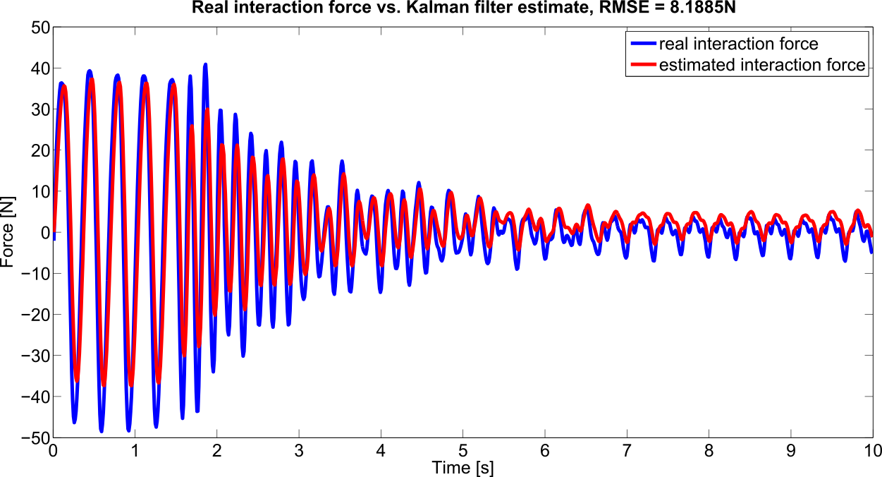The remaining experiments investigated the Kalman filter performance, since interaction force estimation was our main goal. First, we used the data from the previous control experiment to perform offline interaction force estimation. For this, we implemented the previously shown Kalman filter algorithm in a MATLAB script, not using MATLAB's own kalman function to stay as close to the real-time filter as possible. The figure on the left shows the real and the estimated interaction force. We see that, while the estimation amplitude is slightly off, the estimate is very accurate regarding phase and frequency. Since simulation showed the time-related parameters, especially delay, to be much more influential on control performance, this is a good indicator that control could work well using this estimate. 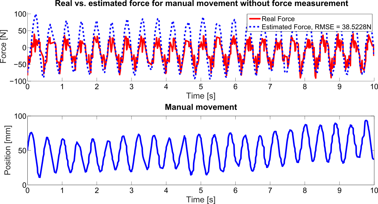For technical reasons we could not perform the full real-time Kalman estimation experiment on the setup and instead implemented a simplified filter on the setup with detached masses. The available measurements were position and force for both masses. For the experiment shown in the right figure, we used the position measurement only to estimate the force. This experiment aimed at showing that a Kalman filter could run in real-time on our setup considering that the matrix operations are costly in terms of computation time. Seeing that this estimator works well even at full 5kHz execution frequency, we are certain that we will be able to use the offline filter in real-time as well. The two Kalman experiments combined show us that a) our Kalman filter is able to estimate interaction force reasonably accurately, especially regarding time-related properties and b) we are able to run our Kalman filter on our setup in real-time, enabling us to use the result for force control.

<latex> {\fontsize{12pt}\selectfont \textbf{Conclusion} </latex>
In conclusion we can say that it is possible to run an efficient transparency controller without having direct access to the interaction force. The most important factors to know for a good estimator model relate to the attachment dynamics. For the controller itself, time-related parameters such as measurement delay or actuator bandwidth are most crucial. If we can account for these main parameters and have a mostly linear system, we can estimate interaction force reasonably well with a conventional Kalman filter. For nonlinear cases, the system might have to be adjusted to use a more sophisticated estimation technique like an extended or unscented Kalman filter. While some situations like the force and acceleration feedback and the combination of the Kalman filter with the controllers still have to be experimented on some further, our simulation results and preliminary experiments show that estimating interaction force in combination with the new control paradigm is a promising approach for accurate transparency control without the need to measure interaction force.