LAB

<latex>{\fontsize{16pt}\selectfont \textbf{Nonlinear Optimal Control}} </latex>
<latex>{\fontsize{16pt}\selectfont \textbf{using Multiple Shooting}} </latex>

<latex>{\fontsize{12pt}\selectfont \textbf{Harsoveet S}} </latex>
<latex>{\fontsize{10pt}\selectfont \textit{Semester Project, RSC}} </latex>

<latex> {\fontsize{12pt}\selectfont \textbf{Abstract} </latex>

One of the challenges that robotics has been facing in the last years is the generation of dynamically feasible trajectories for any general underactuated robotic system. This generation process involves a constrained nonlinear optimization problem and it requires numerical integration to choose a feedforward input in order to obtain the desired trajectories for the system states.

There exist various methods for the generation of these feasible trajectories. One such method is called multiple shooting, which involves breaking down the generation of a single trajectory into the generation of a set of multiple trajectory segments. These segments are then joined through defect constraints in order to produce a single feasible trajectory at the end of the optimization.

This project focuses on implementing trajectory optimization through multiple shooting and comparing the performance against other existing methods. The project also investigates the possibility to extend such methods of trajectory optimization with the ability to handle multiple sets of dynamics within a single optimization.

<latex> {\fontsize{12pt}\selectfont \textbf{Background} </latex>

The traditional optimal control problem attempts to find a set of optimal states and inputs that results in the minimum cost incurred during a particular trajectory. Often, these control problems are constrained to initial/terminal constraints, to path constraints and - of course - must adhere to the ODE model. The equation below shows one such formulation of this problem. This formulation is commonly referred to as trajectory optimization as we are attempting to find the optimal trajectory of the states and controls that minimizes the cost while meeting the constraints.

\begin{equation} \label{eq:optimal_control} \underset{x(.),u(.),T}{\text{minimize}} \int_{0}^{T} l(x(t),u(t)) dt + \phi(x(T)) \end{equation} subject to \begin{equation} \begin{split} \begin{aligned}[c] \notag x(0)-x_0=0,
\dot{x}(t)-f(x(t),u(t))=0,
h(x(t),u(t))\ge 0,
r(x(T))=0
\end{aligned} \qquad\qquad \begin{aligned}[c]
t \in [0,T],
t \in [0,T],

\end{aligned} \qquad\qquad \begin{aligned}[c] \text{(fixed initial value)}
\text{(ODE model)}
\text{(path constraints)}
\text{(terminal constraints)}
\end{aligned} \end{split} \end{equation}

There exist various methods to find the set of optimal controls, but the ones of interest in this project are direct methods. When employing direct methods for the purposes of trajectory optimization, we refer to the problem as direct trajectory optimization.

<latex> {\fontsize{12pt}\selectfont \textbf{Single Shooting} </latex>

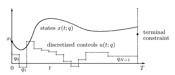
The most straightforward method of direct trajectory optimization is known as single shooting. This is perhaps the most instinctive method that most associate with solving trajectory optimization problems. The system starts as specified by the initial constraint. The controls are then discretized across the time period of interest and the system is integrated forward employing these controls and the ODE model. The controls are then changed according to the gradients in every iteration, ending when all constraints are met (path, initial, terminal) and once a minimum cost is obtained (to a threshold as specified by the user). A visual representation of the single shooting method can be seen below.

<latex> {\fontsize{12pt}\selectfont \textbf{Multiple Shooting} </latex>

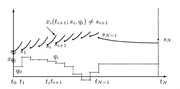
A natural progression to the single shooting method would be to discretize the states as well as the controls. This insight leads to the multiple shooting method; an example of this can be seen below. Once the states are descritized, we can treat each interval as a separate non-linear problem. As such, we are able to integrate all the intervals forward in parallel. To ensure that a feasible trajectory is generated, continuity constraints are imposed such that the end of one interval has the same states as the start of the next interval.

<latex> {\fontsize{12pt}\selectfont \textbf{Direct Transcription} </latex>

The final method for direct trajectory optimization (discussed here) is direct transcription. The multiple shooting and direct transcription methods are quite similar - the direct transcription method also discretizes both the states and the controls. The main difference lies in how the evolution of the system is calculated. The multiple shooting method integrates each interval forward, whereas the direct transcription method employs an approximation (commonly a cubic spline or a trapezoidal method). The same continuity constraint exists, however the direct transcription constraint is more of a defect constraint, as it only approximates the system.

<latex> {\fontsize{12pt}\selectfont \textbf{Software Implementation} </latex>

The multiple shooting class is implemented in a manner similar to the pre-existing Direct Transcription implementation. Much of the logic from this old implementation was moved to a common core, which is now used by both the Direct Transcription and the Multiple Shooting implementations.

For both methods, there are three main elements of importance during the optimization:

<latex> \begin{itemize} \item A parameter vector, listing the components that may be changed during the optimization \item A constraints vector, listing the equations that must be within the stated bounds at the end of the optimization \item The objective function value, which is minimized during the optimization \end{itemize} </latex>

For the multiple shooting implementation, the components of the parameter vector (per shooting period) can be seen below. At each iteration of the optimization, and for every shooting period, this method integrates the states from the start of the period forward employing the dynamics provided by the user. The method uses linear interpolation between the control vector at the start of the current period and the control vector at the start of the following period as inputs during the integration.

<latex> \begin{itemize} \item Length of the period \item State representation at the start of the period \item Control to be employed during the period \end{itemize} </latex>

For the multiple shooting implementation, the components of the constraint vector (per shooting period) can be seen below. As stated previously, the solver attempts to constrain this vector to the bounds chosen by the user. Note that the user may prescribe different bounds to different elements of this vector.

<latex> \begin{itemize} \item Continuity constraint \item Uniform time period constraint (ensures each period is the same length) \item User constraint (passed in during construction of the DTOP object) \item Guard function constraint (if applicable, see Phased Dynamics below) \end{itemize} </latex>

The objective function value is calculated using the definition provided by the user.

<latex> {\fontsize{12pt}\selectfont \textbf{Multiple Shooting vs. Direct Transcription} </latex>

To compare the Mutliple Shooting method against the Direct Transcription method, swing-up trajectories of a double pendulum (also referred to as the acrobot) were generated.

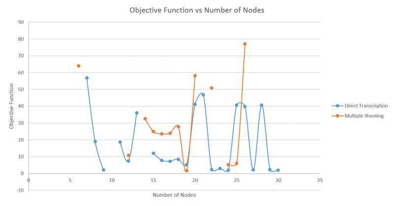
The figure below compares the multiple shooting method against the direct transcription method with respect to the minimized objective function value. As can be seen, the multiple shooting method generally performs worse than the direct transcription method. This can be attributed to the fact that the multiple shooting method integrates the system as opposed to using an approximation. Due to the fact that the direct transcription method generates trajectories that are potentially infeasible in between interval points, when stabilizing these trajectories, a slightly higher gain is required for the direct transcription method as compared to the multiple shooting method.

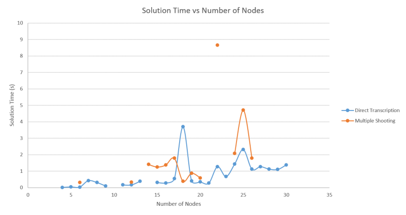
The figure below compares the two methods with respect to the CPU time required for minimization. Once again, the multiple shooting method generally performs worse than the direct transcription method. This can be attributed to the same cause as before - because we are integrating the system as opposed to using an approximation, each iteration of the NLP takes longer.

These results seem to match results in literature, stating that “[multiple shooting has] theoretically higher costs per SQP iteration than collocation”. \cite{diehl}

<latex> {\fontsize{12pt}\selectfont \textbf{Phased Dynamics} </latex>

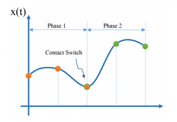
Often in robotics, a multitude of simple dynamics are preferred over a single set of complex dynamics. As can be seen in the figure below, it is possible to decompose one set of dynamics into phases, with the dynamics changing depending on the phase. A common example of this is a single leg of a walking robot: while the leg is in the air, a set of dynamics which do not involve ground forces are dominant, however once the leg lands, the dynamics must change in order to account for ground forces preventing the leg from going through the surface.

To be able to correctly implement phased dynamics, the algorithm must have knowledge of when a phase switch should occur. Although some literature exists for the generation of optimal switching sequences, the topic is still being researched. For the purposes of this project, we assume that the user has a priori knowledge regarding how many phases are required and which dynamics need to be applied during each phase.

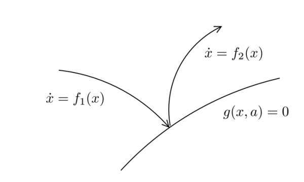
Another issue which arises when implementing phased dynamics is the fact that when a switching of dynamics occurs, we often require that a set of conditions be met. For our walking robot example, we would require that the bottom of the foot has touched the ground before switching between two sets of dynamics. To be able to account for this added constraint, <latex>\emph{guard functions}</latex> are used. During the point of contact between two phases, the relevant guard function must be met (see figure below). As such, a single guard function per phase boundary is required.

<latex> {\fontsize{12pt}\selectfont \textbf{Software Implementation} </latex>

A user may invoke phased dynamics by passing in a vector of dynamics objects as an input to the relevant constructor (as opposed to a single dynamics object). For example, the user may declare three different dynamics, and push back each of these into a vector in the order in which they occur (first-in-first-out). If phased dynamics is requested, a mapping between the shooting periods and the current phase number is generated. This mapping is chosen according to a percentage split specified by the user (eg. 35%/40%/25%). This mapping is then used for all subsequent references to the dynamics, ensuring that the correct set of dynamics is used for each shooting period.

<latex> {\fontsize{10pt}\selectfont \textbf{Example} </latex>
To illustrate the use of phased dynamics, we consider a simple three phase system. In all three phases, the states remain the same:

\begin{equation} x = \begin{bmatrix} x\text{-}pos
z\text{-}pos
angle
x\text{-}vel
z\text{-}vel
anglular\text{ }vel \end{bmatrix} \text{\hspace{25pt}} \label{eq:states} \end{equation}

The meaning of the controls change between phases:

<latex> \begin{itemize} \item[Phase A] Cart-Pole: $ u = \begin{bmatrix} x\text{-}accel \end{bmatrix}$ \item[Phase B] Space Shuttle with Thrust: $ u = \begin{bmatrix} \text{(non-negative) }thrust\text{ }in\text{ }direction\text{ }of\text{ }angle \end{bmatrix}$ \item[Phase C] Object in Freefall: $ u = \begin{bmatrix} unused \end{bmatrix}$ \end{itemize} </latex>

Note that we only require that the state/control vector sizes remain constant - the representation and use thereof may vary between phases, as is the case here for our controls. An optimal trajectory is first generated with no guard functions, using the following conditions:

<latex> \begin{itemize} \item Initial Condition – distance 0, height 0, pole down \item Guard A $\rightarrow$ B – None \item Guard B $\rightarrow$ C – None \item Final Condition – distance 16, height 2, other states of no concern \end{itemize} </latex>

The resulting trajectory can be seen below. A change in color denotes a change in phase.

An optimal trajectory is then generated with guard functions, using the following conditions:

<latex> \begin{itemize} \item Initial Condition – distance 0, height 0, pole down \item Guard A $\rightarrow$ B – distance = 3, velocity = 0 \item Guard B $\rightarrow$ C – height = 10 \item Final Condition – distance 16, height 2, other states of no concern \end{itemize} </latex>

The resulting trajectory can be seen below. As can be seen, the angle cannot be 90 when reaching the phase A $\rightarrow$ B transition, in order to apply the acceleration in the correct direction. The points marked on the animation indicate constraints on the problem (guard functions and terminal constraint).