LAB

<latex>{\fontsize{16pt}\selectfont \textbf{Robot Motion Synthesis using Direct Methods for Trajectory Optimization}} </latex>

<latex>{\fontsize{12pt}\selectfont \textbf{Lukas Möller}} </latex>
<latex>{\fontsize{10pt}\selectfont \textit{Semester Project, EE}} </latex>

<latex> {\fontsize{12pt}\selectfont \textbf{Abstract} </latex>

Similar to optimal control, trajectory optimization deals with finding an open-loop control action such that a specific function is minimized. Furthermore, some prescribed bounds on the input and/or on the states must be fulfilled. In addition to that, within the framework of trajectory optimization, one can also define some path constraints. The function to be minimized, is also denoted as objective function or performance-measure. In this project a general continuous-time nonlinear dynamical system described by first- order nonlinear ODEs is considered. Several numerical methods exist for solving such trajectory optimization problems¹⁾, however only the direct collocation method is investigated here. In recent years, this method became more attractive because of the rising computational power of todays computers. Generally, the trajectory optimization problem is infinite dimensional. With direct collocation one obtains a finite dimensional approximation of that trajectory optimization problem. This approximation is a Nonlinear Program (NLP) which then can be solved with a standard (sparse) numerical NLP solver.
In this project, different collocation methods were studied, where two very well known collocation schemes are chosen for further investigations. The first is the so called Trapezoidal method²⁾ and the second is denoted as the Hermite-Simpson method ³⁾. Furthermore, two NLP-solver were compared. First of all, we considered IPOPT⁴⁾ which is using an Interior-Point method and the second solver is called SNOPT⁵⁾ which implements a Sequential Quadratic Programming method.

<latex> {\fontsize{12pt}\selectfont \textbf{Background} </latex>

The optimal control inputs $u(t)$ are found by minimizing the objective function $$\text{J}(u(t)) = \int_{t_0}^{t_f} \text{J}_{L}(y(t),u(t), t) \mathrm{d}t + \text{J}_{M}(y(t_f), u(t_f), t_f)$$ with its Lagrangian and Mayer term, subject to some dynamical constraints arising from the system dynamics $$\frac{\mathrm{d}y(t)}{\mathrm{d}t} = \mathrm{F}(y(t), u(t), t) \;, \quad y(t_0) = y_{0} \;, \quad y(t_f)= y_{f}$$ as well as bounds on the state $y(t)$ and input $u(t)$ $$\text{y}_l \leq y(t) \leq \text{y}_u$$ $$\text{u}_l \leq u(t) \leq \text{u}_u \text{.}$$ In addition to state and input bounds, we define path constraints of the form $$\text{g}_l \leq \text{g}(u(t), y(t), t) \leq \text{g}_u \text{.}$$ Together, all terms from above, represent the trajectory optimization problem in a mathematical way. Due to the infinite dimensional size, it is convenient to approximate the problem. Therefore we use the method of direct transcription. This leads to a finite dimensional NLP of the form \begin{equation*} \begin{aligned} & \underset{x}{\text{minimize}} & & \text{f}(x)
& \text{subject to} & & \text{g}_{l} \leq \text{g}(x) \leq \text{g}_u
& & & \text{x}_l \leq x \leq \text{x}_u\;\text{,} \end{aligned} \end{equation*} which is large but fortunately sparse. A sparse NLP-solver can then be used to numerically solve the approximate trajectory problem, i.e. the NLP.
In short, we obtain an NLP by discretizing the trajectory optimization problem at N number of nodes along the time horizon $[t_0, t_f]$. The key is, that the dynamical constraints of the system are directly transcribed by using direct collocation. As a result, defect constraints for each interval representing the dynamics, are obtained.

<latex> {\fontsize{12pt}\selectfont \textbf{Trajectory Stabilization} </latex>

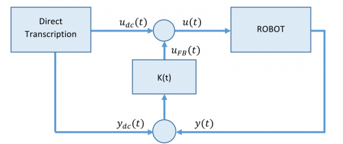
The solution of the NLP is a state and input trajectory which we denote as $y_{dc}(t)$ and $u_{dc}(t)$ respectively. However, the input $u_{dc}(t)$ applied to the system, in general leads to a different state trajectory then $y_{dc}(t)$. The reason is, that the NLP solution is only an approximation as the continuous dynamics are collocated. Hence a stabilizing controller is needed. Therefore a time-varying linear quadratic regulator⁶⁾ (TV-LQR) is chosen. At each time step along the time horizon, the nonlinear dynamics are linearised around the current optimal trajectory and a standard LQR problem is solved. This leads to the feedback law

$$u(t) = u_{dc}(t) - K(t) (y(t) - y_{dc}(t))\;\text{,}$$

where $K(t)$ are the gains, determined by solving the LQR. A block diagram illustrating the control loop is shown in the figure above.
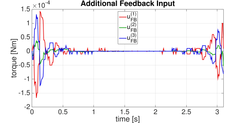
The additional input which steers the state $y(t)$ to the desired nominal state $y_{dc}(t)$ is presented in the plot below. The example was a go-to task which is described in the section “Dynamical System and Benchmark Tasks”. This additonal torques are very small, although necessary in order to keep the system stable and to reach the desired final state $y_f$.

<latex> {\fontsize{12pt}\selectfont \textbf{Software} </latex>

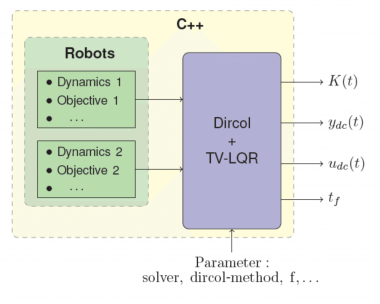
One part of the project was the contribution to a software for solving trajectory optimization problems. The image on the right shows the block diagram of that software. The green block represents some robots with the dynamics, objective function, path constraints etc., which the user of the software has to provide. The purple block, consists of an object which transcribes the trajectory optimization problem into an NLP as well as an object for simulating the system and calculating the feedback gains $K(t)$ for the TV-LQR.
The contribution to the software, was first of all, the implementation of the Trapezoidal collocation method and exploiting sparsity of the NLP when using Hermite-Simpson collocation. Secondly, the continuous cost function of the trajectory optimization problem is now approximated with an appropriate quadrature formula. Thirdly, the software now also supports the NLP-solver IPOPT. Lastly, an object for adding nonlinear path constraints has been added.

<latex> {\fontsize{12pt}\selectfont \textbf{Dynamical System and Benchmark Tasks} </latex>

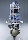
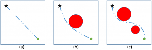
For all investigations, the system dynamics of the unstable robot named Rezero⁷⁾ were used. A picture of the robot is shown below this paragraph on the left. The dimensions of the robot’s state is 10 and it is controlled with 3 inputs. Three tasks are chosen in order to evaluate the performance of the solver and the direct collocation methods. The first and most simple task a) is a go-to task. In the second task b), a cylindrical object is placed between the start and final location. For the last task c) denoted as slalom, the robot has to avoid two different cylindrical objects. All three tasks are qualitatively depicted below in the right figure, with increasing complexity from left to right.

<latex> {\fontsize{12pt}\selectfont \textbf{Experiments} </latex>

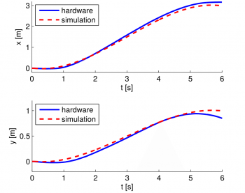
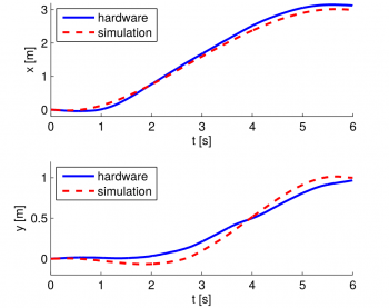
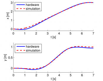
During the project some experiments with the help of two PhD. students (Michael Neunert and Alexander Winkler) on the real robot have been done. The figures below show the experiment's results of all three tasks, starting with task a) on the upper left. On the right task b) is depicted whereas the picture on the bottom illustrates the experiment of the most complex task c). The x and y location of the robot in the two-dimensional plane is shown on the vertical axis of the figure, whereas the horizontal axis illustrates the physical time, starting from 0 seconds up to 6 seconds. For comparison, both the simulated trajectory as well as the measured trajectory are shown in the same figure, as a red dashed line and blue solid line, respectively. The measured trajectory, is the actual trajectory of the hardware, i.e. the real robot.

<latex> {\fontsize{12pt}\selectfont \textbf{Conclusions} </latex>

A very good approximation, in terms of objective value and accuracy of the solution can be achieved, with a small number of nodes. The advantage thereby is, that the NLP does not get too large and the solver might be able to find a solution within a shorter amount of time. Furthermore, it is apparent, that the Hermite-Simpson method is by far more accurate then the Trapezoidal method for a fixed number of Nodes. Regarding the solver, it seems that for robotic problems, Interior-Point solver IPOPT is a promising alternative to the well know SQP solver SNOPT. For increasing complex problems, SNOPT needs more additional time to solve the problem then IPOPT. The solver IPOPT was almost always able to find a feasible solution of the NLP a way faster then SNOPT. On top of that, it was apparent, that the choice of the NLP initialization is crucial for more complex problems. While for the go-to task, the all-zero initialization led to a feasible solution, for the obstacle avoidance tasks “better” initialization methods were very important.