LAB

<latex>{\fontsize{16pt}\selectfont \textbf{Neuromechanics of position/orientation control in planar movements }} </latex>

<latex>{\fontsize{12pt}\selectfont \textbf{[Pascale Meier]}} </latex>
<latex>{\fontsize{10pt}\selectfont \textit{[Master Project ME]}} </latex>

<latex> {\fontsize{12pt}\selectfont \textbf{Abstract} </latex>

Robotics gets more and more important nowadays, they help us to complete work in a more efficient and more economic way. The holy grail of robotics would be to have a self-learning robot so that the only thing one had to do was to assign the desired task to it and the therefore necessary tools. One way to accomplish that is to investigate human learning behaviour in a first step. Naturally, depending on the task a human might follow different strategies. In this work the assignment consisted of a reaching task where subjects had to move their end effector from one point to another as fast and as accurate as possible. It was observed that after several trials, where it can be assumed that the test subjects already learnt this task, the velocity profile had an asymmetric shape. One hypothesis was that these could be described as an overlap of several submovements. In order to reproduce and simulate them a control structure was designed representing a human's motor system while the gains and the inputs that led to the reference trajectories were learned by the Reinforcement Algorithm called <latex>\textit{PI2}</latex> .

<latex> {\fontsize{12pt}\selectfont \textbf{PI2} </latex>
The algorithm called Policy Improvement with Path Integrals (PI2) has its roots in finding path integral solutions to stochastic optimal control problems and is based on solving the Hamilton-Jacobi-Bellman (HJB) equation by using samples in order to obtain the optimal control inputs. It has been shown that <latex>\textit{PI2}</latex> has an efficient performance and results in a very simple form. The only open tuning parameters are the exploration noise and the user-defined cost equations.

As shown in the Figure below the control inputs to the system have the form of \begin{equation}u(t,x) = \Theta^T \Psi(t,x)\end{equation} where <latex>$\Theta^T$</latex> denotes the parameter matrix and $\Psi(t,x)$ a base function vector since <latex>\textit{PI2}</latex> uses function approximation. Therefore, the parameter matrix has to be learned while every column corresponds to a control input. For simplicity it will be assumed from now on that only one control input is present.

The algorithm stops if the change in cost falls below a certain threshold or after exceeding a predefined number of iterations. During every update step the parameter vector gets perturbed in order to explore the surrounding of the current nominal trajectory that results by using the current policy. Thus, K sample rollouts are generated while every rollout is associated with a certain cost. Each rollout contributes something to the parameter update but rollouts that resulted in having a lower cost than others are assigned with a higher probability resp. weight. Since the size of <latex>$\theta^T$</latex> depends on how many base functions are used and on how large the state vector is a weighted averaging needs to be done because currently there is a <latex>$\delta \theta$</latex> for every time step. Afterwards, the update can be performed by <latex>$\theta_{new} = \theta + \delta \theta $</latex>.

<latex> {\fontsize{12pt}\selectfont \textbf{Control Structure and Arm Model} </latex>
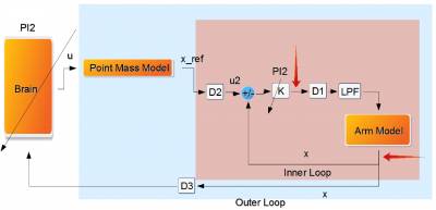
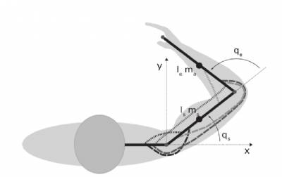
The control structure as shown in Figure 2 represents a human's motor system. Therefore, it is divided into an inner loop that represents a human's arm and an outer loop that corresponds to a human's motion phase. Both loops use <latex>\textit{PI2}</latex> for learning the gains resp. the inputs that provided the reference trajectory to the arm model. The inner loop consists of a muscle activation delay block of ca. <latex>\unit[5]{ms}</latex> which is the time that is needed for the muscle spindles to fire, a muscle-like Low Pass filter and a transmission delay block of ca. <latex>\unit[50]{ms}</latex>. Since it has been shown that the noise in our motor system is of multiplicative nature such a noise is added to the inner loop as well. On the other hand the outer loop contains a vision delay block and also a velocity-dependent multiplicative noise source (red arrow) since it is assumed that our measurements become noisier when increasing the speed of our end effector. Furthermore, a 2-link arm model was supposed as shown in Figure 3 using anthropometric data.

<latex> {\fontsize{12pt}\selectfont \textbf{Results} </latex>
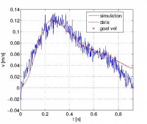
Firstly, only a point mass model was assumed. Since the submovements couldn't be reproduced by just using a velocity-dependent noise source that should simulate the increase and decrease of the end effector's velocity due visual corrections the cost function was adapted as followed: On one hand a deviation between current and desired end position got penalized in order to move there fast which was one requirement of the reaching task experiments. On the other hand the subjects had to be accurate when approaching the goal position. Therefore, the distance between start and end position was divided in two segments. At the beginning accuracy isn't an issue, thus the movement can be fast and velocity is cheap. Afterwards, when exceeding a certain position threshold accuracy matters, thus it is necessary to slow down resp. velocities get penalized stronger than before. The results are shown in Figure 4 \begin{equation}

   \begin{aligned}
    &l(x(t),u(t)) := K_0 \dot{x}^2 + 1000(x - x_{goal})^2 + 500(\dot{x} -\dot{x}_{goal})^2\\

&h(x(t_f)) := 2000(x - x_{goal})^2 + 50(\dot{x} -\dot{x}_{goal})^2
&K_0 :=

\begin{cases}
 2 & \text{if } x \leq 0.5|x_0 - x_{goal}| + x_0 \\
 20       & \text{else} 
\end{cases}
   \end{aligned}

\end{equation}

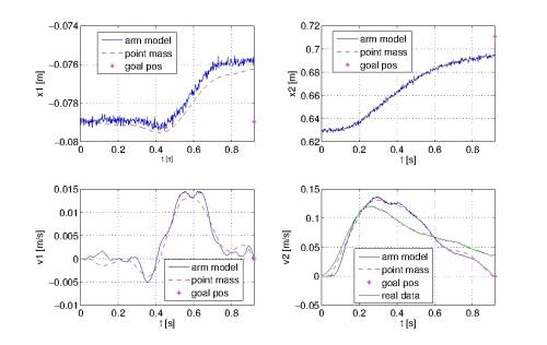
The same was done after in combination with the arm model. The corresponding results are shown in Figure 5. Furthermore, in order to handle singularities and to provide smooth movements \textit{Operational Space Control} was used.

Hence, a combination of penalizing deviations to the end position and considering the its variability depending on where the end effector is located yielded the desired submovements.